Kerr Newman Metrik

[Yukterez]

Das ist die deutschsprachige Version.   English versions are available on en.yukterez.net and here.

Verwandte Beiträge: KNdS || SSdS || Kerr || Schwarzschild || Feldgleichungen || Gravitationslinsen || Raytracing || Flamm  
 

  ←
Akkretionsscheibe um ein geladenes und rotierendes SL mit a=0.95, ℧=0.3, ri=isco, ra=10, Blickwinkel=89°. Erdoberfläche auf r=1.01r+.    
 

  ←
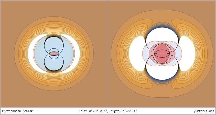
Kretschmann Skalar, kartesische Projektion, Blickwinkel=90°. Die Bereiche um die Pole sind negativ, und jene um den Äquator positiv gekrümmt.    
 

  ←
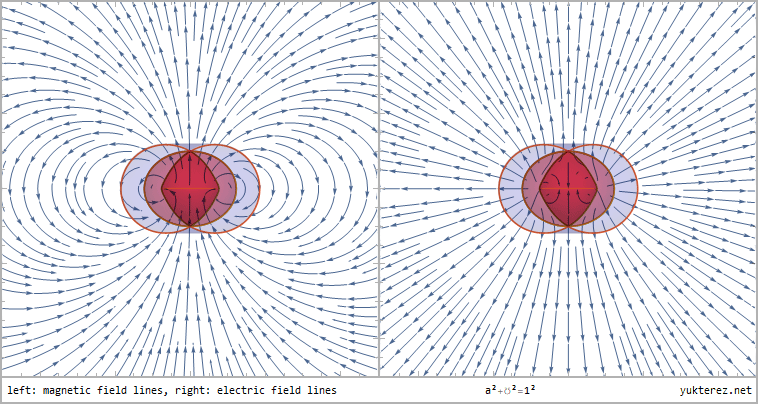
Magnetische (links) und elektrische (rechts) Feldlinien, kartesische Projektion, Blickwinkel=90° (edge on), Plotbereich=±5.    
 

  ←
Retrograder Orbit eines mit q=1 geladenen Partikels um ein SL mit a=√¾ & ℧=⅓. v0 & i0: lokale Startgeschwindigkeit & Inklination    

  ←
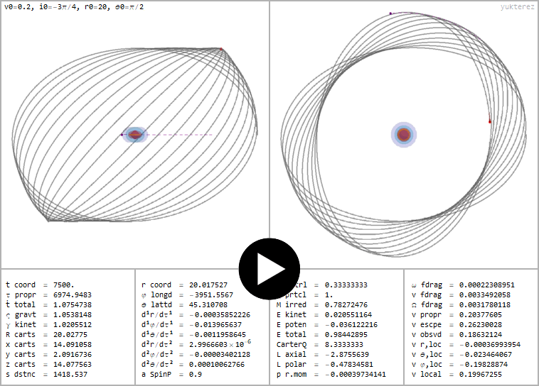
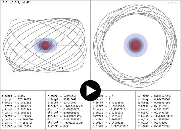
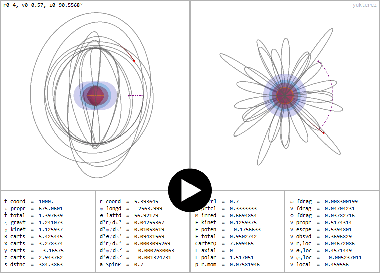
Prograder Orbit eines neutralen Testpartikels um ein mit a=0.9 rotierendes und ℧=0.4 elektrisch geladenes Kerr Newman SL    

  ←
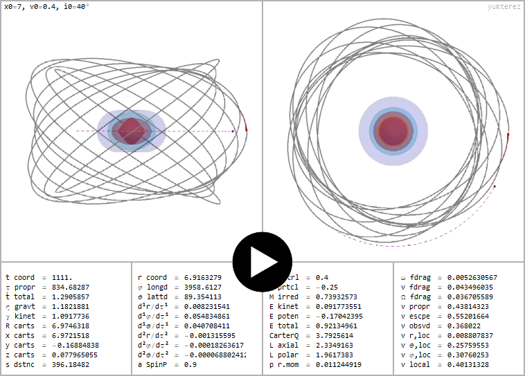
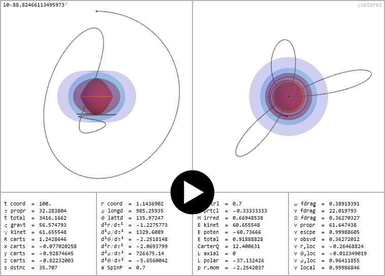
Prograder Orbit eines negativ geladenen Testpartikels (q=-¼) um ein wie oben rotierendes und positiv geladenes schwarzes Loch    

  ←
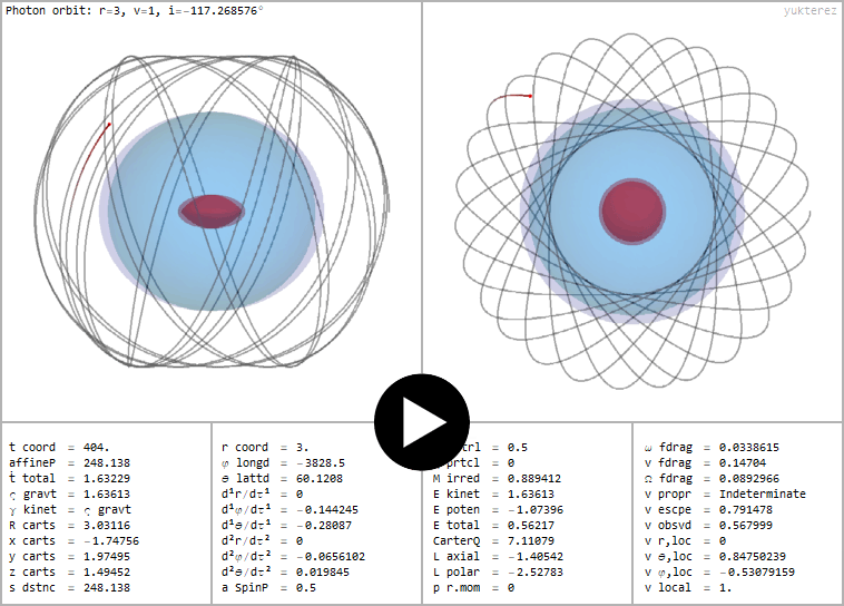
Nichtäquatorialer und retrograder Photonenorbit um ein mit a=½ und ℧=½ geladenes schwarzes Loch, konstanter Boyer Lindquist Radius      

  ←
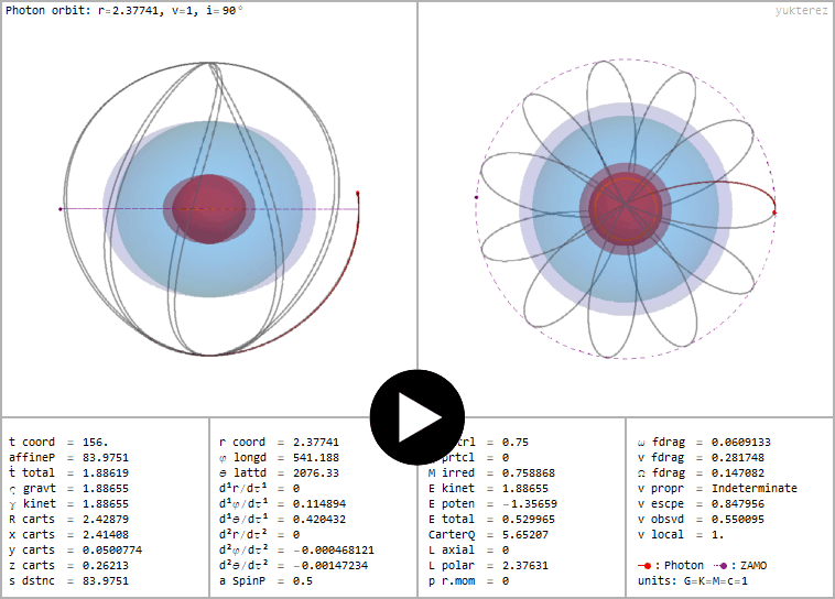
Polarer Photonenorbit (Lz=0) um ein mit a=½ rotierendes und mit ℧=¾ geladenes schwarzes Loch, konstanter Boyer Lindquist Radius      

  ←
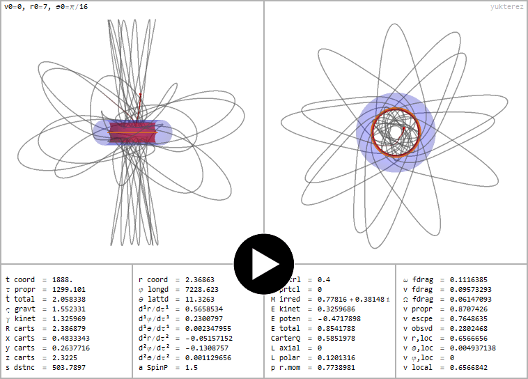
Polarer Orbit (Lz=0) eines positiv geladenen Testpartikels (q=⅓) um ein positiv geladenes und rotierendes schwarzes Loch (℧=a=0.7)    

  ←
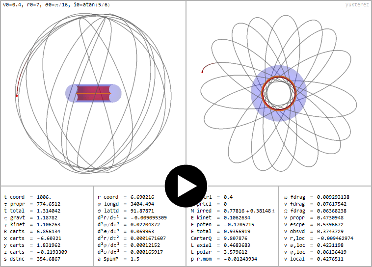
Plunge Orbit eines negativen Teilchens (q=-⅓), SL wie oben. Die Axialgeschwindigkeit bei q<0 ist für Lz=0 wegen der elektrischen Kraft positiv.    

  ←
Freier Fall eines neutralen Testpartikels auf eine mit mit a=1.5 rotierende und und ℧=0.4 elektrisch geladene nackte Singularität      

  ←
Geodätischer Orbit um eine nackte Singularität mit den gleichen Spin- und Ladungsparametern wie ein Beispiel weiter oben    
 

  ←
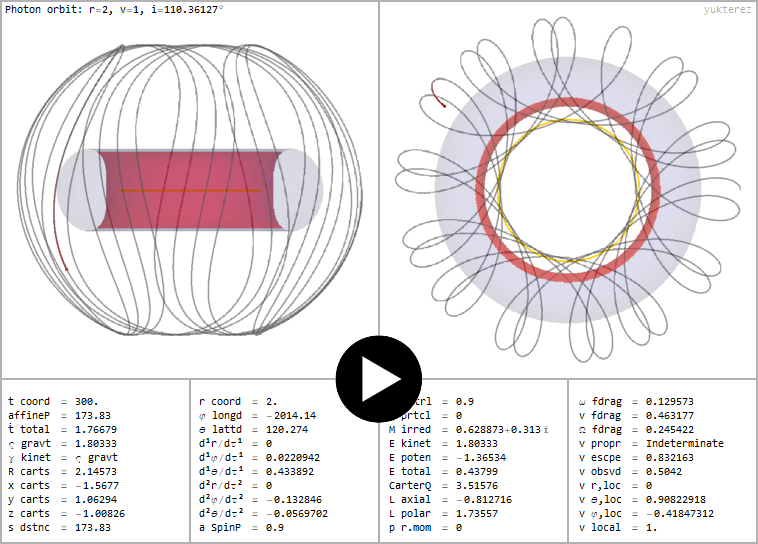
Nichtäquatorialer und retrograder Photonenorbit um eine mit a=0.9 rotierende und ℧=0.9 geladene nackte Singularität    
 

  ←
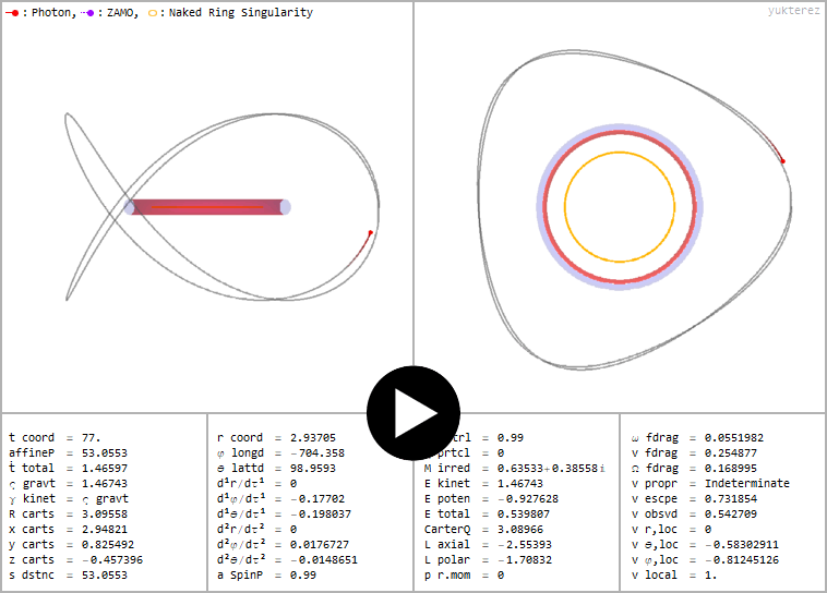
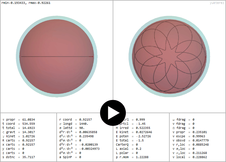
Retrograder Photonenorbit um eine nackte Singularität (a=0.99, ℧=0.99). Lokale äquatoriale Inklination: -2.5rad=-143.23945°    
 

  ←
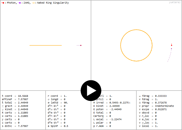
Stationärer Photonenorbit (E=0) um eine Ringsingularität (a=½, ℧=1). Außer bei r=1, θ=90° ist v framedrag überall <c, daher keine Ergosphären.      

  ←
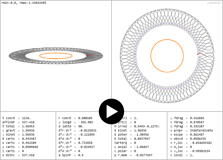
Äquatorialer retrograder Photonenorbit, Singularität bei r=0→R=√(r²+a²)=a=½. Ergoring (rosa) bei r=1, Umkehrpunkte bei r=0.8 und r=1.3484      

  ←
Orbit eines negativ geladenen Partikels innerhalb des Cauchy Horizonts eines Reissner Nordström SL (vergleiche Dokuchaev, Fig. 1)      

[Yukterez]

Linienelement in Boyer-Lindquist-Koordinaten, metrische Signatur (+,-,-,-):



zusammengefasste Terme:



mit dem Spinparameter â=Jc/G/M bzw. dem dimensionslosen Spinparameter a=â/M und dem elektrischen Ladungsparameter Ω=⚼·√(K/G) bzw. dem dimensionslosen spezifischen Ladungsparameter ℧=Ω/M. Der Artikel verwendet die dimensionslosen natürlichen Einheiten G=M=c=K=ℏ=1 mit Längen in GM/c² und Zeiten in GM/c³. Der Zusammenhang zwischen dem hier gleich 1 gesetzten Massenäquivalent M und der irreduziblen Masse Mirr ist



Effektive Masse (wo diese 0 ist wird auch die Beschleunigung 0):



Für massebehaftete Testpartikel gilt μ=-1, für Photonen μ=0. Die spezifische Ladung des Testpartikels ist q. Transformationsregel für ko-und kontravariante Indizes (hochgestellte Buchstaben sind hierbei keine Potenzen sondern Indizes):



Ko- und kontravariante Metrik:

Elektromagnetisches Potential:



Kovarianter elektromagnetischer Tensor:



Kontravarianter Maxwelltensor:



Magnetische Feldlinien:



Elektrische Feldlinien:



wobei



Mit den Christoffelsymbolen



lauten die zweiten Eigenzeitableitungen der Koordinaten:



Damit lauten die Bewegungsgleichungen:









Zusammenhang zwischen dem kanonischen Viererimpuls, der lokalen Dreiergeschwindigkeit und den ersten Eigenzeitableitungen:

Aus dem Linienelement:



gewonnene Zeitdilatation eines neutralen Testpartikels:



Insgesamte Zeitdilatation eines geladenen Testpartikels:



Zusammenhang der ersten Eigenzeitableitungen mit den kovarianten Impulskomponenten:





Zusammenhang der ersten Eigenzeitableitungen mit den lokalen Dreiergeschwindigkeitskomponenten:

   



mit dem kontrahierten transversalen elektromagnetischen Potential



Das radiale effektive Potential das an seinen Nullstellen die Umkehrpunkte vorgibt ist



und das latitudinale Potential



mit dem Parameter



Für die lokale Dreiergeschwindigkeit relativ zu einem ZAMO vor Ort wird E nach v aufgelöst:



oder die gravitative Zeitdilatation durch die gesamte Zeitdilatation dividiert um den Kehrwert des Gammafaktors zu erhalten:



Radiale Fluchtgeschwindigkeit für ein neutrales Teilchen:



Für die Fluchtgeschwindigkeit eines drehimpulsfreien geladenen Teilchens wird E=1 gesetzt und nach v aufgelöst:

1. Erhaltungsgröße: Gesamtenergie E=-pt

2. Erhaltungsgröße: axialer Drehimpuls Lz=+pφ

3. Erhaltungsgröße: Carter-Konstante



mit der koaxialen Drehimpulskomponente (die selber keine Erhaltungsgröße ist)



Radiale Impulskomponente:



Die azimutalen und latitudinalen Stoßparameter sind



Gravitative Zeitdilatation eines ZAMO, unendlich am Horizont:



Zeitdilatation eines neutralen stationären Partikels, unendlich bei der Ergosphäre:

Frame-Dragging Winkelgeschwindigkeit im System den Koordinatenbuchhalters:



Lokale Frame-Dragging Geschwindigkeit relativ zu den Fixsternen (bei der Ergosphäre c):



Axialer und koaxialer Gyrationsradius:



Axialer und koaxialer Umfang:



Die Radien der äquatorialen Photonenkreisorbits sind implizit gegeben durch:

Der letzte stabile Orbit (ISCO) eines neutralen Partikels ergibt sich aus:



Radialkoordinaten der Horizonte und Ergosphären:



Kartesische Projektion:



r in Relation zu x,y,z:



Kartesischer Radius:



Kartesischer Breitengrad:



Hawking Temperatur (mit Surface Gravity κ⁺):



Andere Koordinaten: hier entlang

[Yukterez]

Transformationsregel von Boyer Lindquist auf Doran Raindrop:



Der Raumfluss hat relativ zu einem lokalen ZAMO die negative radiale Fluchtgeschwindigkeit:

Metrischer Tensor in Doran Raindrop Koordinaten, kovariant:



Kontravarianter metrischer Tensor:



Elektromagnetisches Potential:



Kovarianter Maxwelltensor:



Kontravarianter elektromagnetischer Tensor:



Gesamtgeschwindigkeit relativ zu einem lokalen Regentropfen:



Radiale lokale Geschwindigkeit:



Latitudinale lokale Geschwindigkeit:



Longitudinale lokale Geschwindigkeit:



Zeitdifferential:







Mehr Details: hier entlang, Vergleich Boyer Lindquist mit Raindrop Doran (Animation und Plots): klick, Sicht aus dem Inneren eines schwarzen Lochs: klick, andere Koordinaten: Liste

[Yukterez]

1) Input: Linienelement und Maxwell-Tensor in Boyer Lindquist Koordinaten, Output: Bewegungsgleichungen

Code: Alles auswählen

(* |||||||||||||||||||||||||||||||||||||||||||||||||||||||||||||||||||||||||||||||||||||| *)
(* | Mathematica Syntax | GEODESIC SOLVER | geodesics.yukterez.net | Version 21.01.2020 | *)
(* |||||||||||||||||||||||||||||||||||||||||||||||||||||||||||||||||||||||||||||||||||||| *)

ClearAll["Local`*"]; ClearAll["Global`*"];
smp[y_]:=Simplify[y, Reals]; list[y_]:=y[[1]]==y[[2]];
rplc[y_]:=(((((((y/.t->t[τ])/.r->r[τ])/.θ->θ[τ])/.φ->φ[τ])/.Derivative[1][t[τ]]->
t'[τ])/.Derivative[1][r[τ]]->r'[τ])/.Derivative[1][θ[τ]]->θ'[τ])/.Derivative[1][φ[τ]]->φ'[τ]

                                                      (* kovariante metrische Komponenten *)
g11=gtt=-((-Δ+ж a^2 Sin[θ]^2)/(Σ χ^2));
g22=grr=-Σ/Δ;
g33=gθθ=-Σ/ж;
g44=gφφ=-((ж σ^2 Sin[θ]^2-a^2 Δ Sin[θ]^4)/(Σ χ^2));
g14=gtφ=-(( a (Δ-ж σ) Sin[θ]^2)/(Σ χ^2));
g12=g13=g23=g24=g34=0;

                                                                           (* Abkürzungen *)
Σ=r^2+a^2 Cos[θ]^2;
Δ=(r^2+a^2)(1-Λ/3 r^2)-2 M r+℧^2;
Χ=(r^2+a^2)^2-a^2 Sin[θ]^2 Δ;
щ=(q ℧ r (a^2+r^2))/(Δ Σ);
χ=1+Λ/3 a^2;
ж=1+Λ/3 a^2 Cos[θ]^2;
σ=a^2+r^2;

                           (* Dimensionen, elektrische Ladung, Spin, Vakuumenergie, Masse *)
x={t, r, θ, φ}; n=4; Ω=℧; ℧=℧; a=a; Λ=0; M=1;

                                                                         "Metrischer Tensor"
mt={{g11, g12, g13, g14}, {g12, g22, g23, g24}, {g13, g23, g33, g34}, {g14, g24, g34, g44}};
Subscript["g", μσ] -> MatrixForm[mt]
it=smp[Inverse[mt]];
"g"^μσ -> MatrixForm[it]

                                                                            "Maxwell Tensor"
A={Ω r/Σ/χ, 0, 0, -Ω r/Σ/χ Sin[θ]^2 a};
F=smp[Table[((D[A[[j]], x[[k]]]-D[A[[k]], x[[j]]])), {j, 1, n}, {k, 1, n}]];
Subscript["F", μσ] -> MatrixForm[F]
f=smp[Table[Sum[
it[[i, k]] it[[j, l]] F[[k, l]],
{k, 1, n}, {l, 1, n}], {i, 1, n}, {j, 1, n}]];
"F"^μσ -> MatrixForm[f]

                                                                        "Christoffelsymbole"
chr=smp[Table[(1/2)Sum[(it[[i, s]])
(D[mt[[s, j]], x[[k]]]+D[mt[[s, k]], x[[j]]] -D[mt[[j, k]], x[[s]]]), {s, 1, n}],
{i, 1, n}, {j, 1, n}, {k, 1, n}]];
crs=Table[If[UnsameQ[chr[[i, j, k]], 0],
{ToString[Γ[i, j, k]] "\[Rule]", chr[[i, j, k]]}], {i, 1, n}, {j, 1, n}, {k, 1, j}];
TableForm[Partition[DeleteCases[Flatten[crs], Null], 2]]
                 
                                                                 "gemischter Riemann Tensor"
rmn=smp[Table[
D[chr[[i, j, l]], x[[k]]] - D[chr[[i, j, k]], x[[l]]] +
Sum[chr[[s, j, l]] chr[[i, k, s]] -
chr[[s, j, k]] chr[[i, l, s]],
{s, 1, n}], {i, 1, n}, {j, 1, n}, {k, 1, n}, {l, 1, n}]];
rie=Table[If[UnsameQ[rmn[[i, j, k, l]], 0],
{ToString[R[i, j, k, l]] "\[Rule]", rmn[[i, j, k, l]]}],
{i, 1, n}, {j, 1, n}, {k, 1, n}, {l, 1, k - 1}];
TableForm[Partition[DeleteCases[Flatten[rie], Null], 2]]
                                                            (* kovarianter Riemann Tensor *)
rcv=Table[Sum[mt[[i, j]] rmn[[j, k, l, m]], {j, 1, 4}],
{i, 1, n}, {k, 1, n}, {l, 1, n}, {m, 1, n}];
                                                        (* kontravarianter Riemann Tensor *)
rcn=Table[Sum[it[[m, i]] it[[h, j]] it[[o, k]] it[[p, l]] rcv[[i, j, k, l]],
{i, 1, 4}, {j, 1, n}, {k, 1, n}, {l, 1, n}],
{m, 1, 4}, {h, 1, n}, {o, 1, n}, {p, 1, n}];

                                                                              "Ricci Tensor"
rcc=smp[Table[
Sum[rmn[[i, j, i, l]], {i, 1, n}], {j, 1, n}, {l, 1, n}]];
Subscript["Ř", μσ] -> MatrixForm[rcc]
ric=smp[Table[Sum[
it[[i, k]] it[[j, l]] rcc[[k, l]], {k, 1, n}, {l, 1, n}],
{i, 1, n}, {j, 1, n}]];
"Ř"^μσ -> MatrixForm[ric]

                                                                              "Ricci Skalar"
Ř=smp[Sum[it[[i, j]] rcc[[i, j]], {i, 1, n}, {j, 1, n}]]; "Ř"->Ř

                                                                        "Kretschmann Skalar"
krn= Sum[rcv[[i, j, k, l]] rcn[[i, j, k, l]],
{i, 1, 4}, {j, 1, n}, {k, 1, n}, {l, 1, n}];
"K"->smp[krn]

                                                                           "Einstein Tensor"
est=smp[rcc-Ř mt/2];
Subscript["G", μσ] -> MatrixForm[est]
ein=smp[Table[Sum[
it[[i, k]] it[[j, l]] est[[k, l]], {k, 1, n}, {l, 1, n}],
{i, 1, n}, {j, 1, n}]];
"G"^μσ -> MatrixForm[smp[ein]]

                                                                     "Stress Energie Tensor"
set=smp[est-Λ mt]/8/π;                                                   
Subscript["T", μσ] -> MatrixForm[set]
sei=smp[Table[Sum[
it[[i, k]] it[[j, l]] set[[k, l]], {k, 1, n}, {l, 1, n}],
{i, 1, n}, {j, 1, n}]];
"T"^μσ -> MatrixForm[smp[sei]]

                                                                      "Bewegungsgleichungen"
geo=smp[Table[-Sum[
chr[[i, j, k]] x[[j]]' x[[k]]'+q f[[i, k]] x[[j]]' mt[[j, k]],
{j, 1, n}, {k, 1, n}], {i, 1, n}]];

equ=Table[{x[[i]]''[τ]==smp[rplc[geo[[i]]]]}, {i, 1, n}];

geodesic1=equ[[1]][[1]]
geodesic2=equ[[2]][[1]]
geodesic3=equ[[3]][[1]]
geodesic4=equ[[4]][[1]]

                                                                     "totale Zeitdilatation"
H=Sum[mt[[μ, ν]] x[[μ]]' x[[ν]]', {μ, 1, n}, {ν, 1, n}];   
Derivative[1][s][τ]^2 == "ds²/dτ² == -μ" == smp[rplc[H]]                       
ṫ=Quiet[rplc[smp[Normal[Solve[
-μ==(H/.t'->ť), ť]]]]];                       
Derivative[1][t][τ]->ṫ[[1, 1, 2]] || ṫ[[2, 1, 2]]||rplc[Sqrt[it[[1, 1]]]]/Sqrt[1-v[τ]^2]

                                                                  "kovarianter Viererimpuls"
p[μ_]:=-(Sum[mt[[μ, ν]]*x[[ν]]', {ν, 1, n}]+q A[[μ]]);
pt[τ]->rplc[smp[p[1]]]
pr[τ]->rplc[smp[p[2]]]
pθ[τ]->rplc[smp[p[3]]]
pφ[τ]->rplc[smp[p[4]]]

                                                                    "lokale Geschwindigkeit"
V[x_]:=smp[Normal[Solve[vx Sqrt[-mt[[x, x]]]/Sqrt[1-μ^2 v[τ]^2]-(1-μ^2 v^2) q A[[x]]==
p[x], vx]][[1, 1]]];                                                   
rplc[V[2]]/.vx->vr[τ]
rplc[V[3]]/.vx->vθ[τ]
rplc[V[4]]/.vx->vφ[τ]










2) Simulator-Code für Photonen, geladene und neutrale Teilchen in Boyer Lindquist Koordinaten

Code: Alles auswählen

(* Simulator-Code für Photonen, geladene und neutrale Teilchen                            *)
(* in Boyer Lindquist Koordinaten                                                         *)

(* |||||||||||||||||||||||||||||||||||||||||||||||||||||||||||||||||||||||||||||||||||||| *)
(* |||| Mathematica | kerr.newman.yukterez.net | 06.08.2017 - 13.06.2020, Version 25 |||| *)
(* |||||||||||||||||||||||||||||||||||||||||||||||||||||||||||||||||||||||||||||||||||||| *)
 
wp=MachinePrecision;
mt1=Automatic;
mt2={"EquationSimplification"-> "Residual"};
mt3={"ImplicitRungeKutta", "DifferenceOrder"-> 20};
mt4={"StiffnessSwitching", Method-> {"ExplicitRungeKutta", Automatic}};
mt5={"EventLocator", "Event"-> (r[τ]-1001/1000 rA)};
mta=mt1;                                                     (* mt1: Speed, mt3: Accuracy *)
dgl=1;         (* 1: Full d²x/dτ², 2: Mixed dx/dτ, 3: Testmodul, 4: Weak Field, 5: Newton *)
 
(* |||||||||||||||||||||||||||||||||||||||||||||||||||||||||||||||||||||||||||||||||||||| *)
(* |||||||| 1) STARTBEDINGUNGEN EINGEBEN |||||||||||||||||||||||||||||||||||||||||||||||| *)
(* |||||||||||||||||||||||||||||||||||||||||||||||||||||||||||||||||||||||||||||||||||||| *)
 
A=a;                                             (* pseudosphärisch: A=0, kartesisch: A=a *)
 
tmax=300;                                                                    (* Eigenzeit *)
Tmax=300;                                                              (* Koordinatenzeit *)
TMax=Min[Tmax, т[plunge-1/100]]; tMax=Min[tmax, plunge-1/100];        (* Integrationsende *)
 
r0 = Sqrt[7^2-a^2];                                                        (* Startradius *)
r1 = r0+2;                                                   (* Endradius wenn v0=vr0=vr1 *)
θ0 = π/2;                                                                  (* Breitengrad *)
φ0 = 0;                                                                     (* Längengrad *)
a  = 9/10;                                                               (* Spinparameter *)
℧  = 2/5;                                       (* spezifische Ladung des schwarzen Lochs *)
q  = 0;                                             (* spezifische Ladung des Testkörpers *)
 
v0 = 2/5;                                                       (* Anfangsgeschwindigkeit *)
α0 = 0;                                                      (* vertikaler Abschusswinkel *)
i0 = ArcTan[5/6];                                               (* Bahninklinationswinkel *)
 
(* |||||||||||||||||||||||||||||||||||||||||||||||||||||||||||||||||||||||||||||||||||||| *)
(* |||||||| 2) GESCHWINDIGKEITS-, ENERGIE UND DREHIMPULSKOMPONENTEN ||||||||||||||||||||| *)
(* |||||||||||||||||||||||||||||||||||||||||||||||||||||||||||||||||||||||||||||||||||||| *)
 
vr0=v0 Sin[α0];                                     (* radiale Geschwindigkeitskomponente *)
vθ0=v0 Cos[α0] Sin[i0];                      (* longitudinale  Geschwindigkeitskomponente *)
vφ0=v0 Cos[α0] Cos[i0];                        (* latitudinale Geschwindigkeitskomponente *)

vrj[τ_]:=R'[τ]/Sqrt[Δi[τ]] Sqrt[Σi[τ] (1+μ v[τ]^2)];
vθj[τ_]:=Θ'[τ] Sqrt[Σi[τ] (1+μ v[τ]^2)];
vφj[τ_]:=Evaluate[(-(((a^2 Cos[θ[τ]]^2+r[τ]^2) (a^2+℧^2-2 r[τ]+r[τ]^2) Sin[θ[τ]] Sqrt[1-
μ^2 v[τ]^2] (-φ'[τ]-(a q ℧ r[τ])/((a^2 Cos[θ[τ]]^2+r[τ]^2) (a^2+℧^2-2 r[τ]+r[τ]^2))+
(ε Csc[θ[τ]]^2 (a (-a^2-℧^2+2 r[τ]-r[τ]^2) Sin[θ[τ]]^2+a (a^2+
r[τ]^2) Sin[θ[τ]]^2))/((a^2 Cos[θ[τ]]^2+r[τ]^2) (a^2+℧^2-2 r[τ]+r[τ]^2))+(a q ℧ r[τ] (a^2+
℧^2-2 r[τ]+r[τ]^2-a^2 Sin[θ[τ]]^2))/((a^2 Cos[θ[τ]]^2+r[τ]^2)^2 (a^2+℧^2-2 r[τ]+
r[τ]^2) (1-μ^2 v[τ]^2))))/((a^2+℧^2-2 r[τ]+r[τ]^2-a^2 Sin[θ[τ]]^2) Sqrt[((a^2+r[τ]^2)^2-
a^2 (a^2+℧^2-2 r[τ]+r[τ]^2) Sin[θ[τ]]^2)/(a^2 Cos[θ[τ]]^2+r[τ]^2)]))) /. sol][[1]]
vtj[τ_]:=Sqrt[vrj[τ]^2+vθj[τ]^2+vφj[τ]^2];
vr[τ_]:=vrj[τ]/vtj[τ]*v[τ];
vθ[τ_]:=vθj[τ]/vtj[τ]*v[τ];
vφ[τ_]:=vφj[τ]/vtj[τ]*v[τ];
VΦ[τ_]:=Sqrt[v[τ]^2-vθ[τ]^2-vr[τ]^2];
Vφ[τ_]:=If[q==0, Vφ[τ], VΦ[τ]];
 
x0[A_]:=Sqrt[r0^2+A^2] Sin[θ0] Cos[φ0];                             (* Anfangskoordinaten *)
y0[A_]:=Sqrt[r0^2+A^2] Sin[θ0] Sin[φ0];
z0[A_]:=r0 Cos[θ0];
 
ε0=Sqrt[δ Ξ/χ]/j[v0]+Lz ω0;
ε=ε0+((q r0 ℧)/(r0^2+a^2 Cos[θ0]^2));
εζ:=Sqrt[Δ Σ/Χ]/j[ν]+Lz ωζ+((q r[τ] ℧)/(r[τ]^2+a^2 Cos[θ[τ]]^2));
LZ=vφ0 Ы/j[v0];
Lz=LZ+((q a r0 ℧ Sin[θ0]^2)/(r0^2+a^2 Cos[θ0]^2)) j[v0]^2;
Lζ:=vφ0 я/j[ν]+0((q a r[τ] ℧ Sin[θ[τ]]^2)/(r[τ]^2+a^2 Cos[θ[τ]]^2));
pθ0=vθ0 Sqrt[Ξ]/j[v0]; pθζ:=θ'[τ] Σ;
pr0=vr0 Sqrt[(Ξ/δ)/j[v0]^2];
Qk=Limit[pθ0^2+(Lz^2 Csc[θ1]^2-a^2 (ε^2+μ)) Cos[θ1]^2, θ1->θ0];       (* Carter Konstante *)
Q=Limit[pθ0^2+(Lz^2 Csc[θ1]^2-a^2 (ε^2+μ)) Cos[θ1]^2, θ1->θ0];
Qζ:=pθζ^2+(Lz^2 Csc[θ[τ]]^2-a^2 (εζ^2+μ)) Cos[θ[τ]]^2;
k=Q+Lz^2+a^2 (ε^2+μ); kζ:=Qζ+Lz^2+a^2 (εζ^2+μ);
                                                                                  (* ISCO *)
isco = rISCO/.Solve[0 == rISCO (6 rISCO-rISCO^2-9 ℧^2+3 a^2)+4 ℧^2 (℧^2-a^2)-
8 a (rISCO-℧^2)^(3/2) && rISCO>=rA, rISCO][[1]];
μ=If[Abs[v0]==1, 0, If[Abs[v0]<1, -1, 1]];                   (* Baryon: μ=-1, Photon: μ=0 *)

(* |||||||||||||||||||||||||||||||||||||||||||||||||||||||||||||||||||||||||||||||||||||| *)
(* |||||||| 3) FLUCHTGESCHWINDIGKEIT UND BENÖTIGTER ABSCHUSSWINKEL |||||||||||||||||||||| *)
(* |||||||||||||||||||||||||||||||||||||||||||||||||||||||||||||||||||||||||||||||||||||| *)

vEsc=If[q==0, ж0, Abs[(\[Sqrt](r0^2 (r0^2 (δ Ξ-χ)+2 q r0 χ ℧-q^2 χ ℧^2)+
2 a^2 r0 (r0 δ Ξ-r0 χ+q χ ℧) Cos[θ0]^2+a^4 (δ Ξ-
χ) Cos[θ0]^4))/(Sqrt[χ] (r0 (r0-q ℧)+a^2 Cos[θ0]^2))]];
                                                  (* horizontaler Photonenkreiswinkel, i0 *)
iP[r0_, a_]:=Normal[iPh/.NSolve[1/(8 (r0^2+a^2 Cos[θ0]^2)^3) (a^2+(-2+r0) r0+
℧^2) (8 r0 (r0^2+a^2 Cos[θ0]^2) Sin[iPh]^2+1/((a^2-2 r0+r0^2+℧^2) (r0^2+
a^2 Cos[θ0]^2)) 8 a (Cos[iPh] Sin[θ0] (a^2-2 r0+r0^2+℧^2-a^2 Sin[θ0]^2) Sqrt[((a^2+
r0^2)^2-a^2 (a^2-2 r0+r0^2+℧^2) Sin[θ0]^2)/(r0^2+a^2 Cos[θ0]^2)]+(a (a^2+r0^2) Sin[θ0]^2+
a (-a^2+2 r0-r0^2-℧^2) Sin[θ0]^2) (Sqrt[((a^2-2 r0+r0^2+℧^2) (r0^2+a^2 Cos[θ0]^2))/((a^2+
r0^2)^2-a^2 (a^2-2 r0+r0^2+℧^2) Sin[θ0]^2)]+(a (2 r0-℧^2) Cos[iPh] Sin[θ0] Sqrt[((a^2+
r0^2)^2-a^2 (a^2-2 r0+r0^2+℧^2) Sin[θ0]^2)/(r0^2+a^2 Cos[θ0]^2)])/((a^2+r0^2)^2-a^2 (a^2-
2 r0+r0^2+℧^2) Sin[θ0]^2))) (-(1/((a^2-2 r0+r0^2+℧^2) (r0^2+
a^2 Cos[θ0]^2)))2 a^2 Cot[θ0]^2 (Cos[iPh] Sin[θ0] (-a (a^2+r0^2) Sin[θ0]^2+a (a^2-2 r0+
r0^2+℧^2) Sin[θ0]^2) Sqrt[((a^2+r0^2)^2-a^2 (a^2-2 r0+r0^2+℧^2) Sin[θ0]^2)/(r0^2+
a^2 Cos[θ0]^2)]+((a^2+r0^2)^2 Sin[θ0]^2+a^2 (-a^2+2 r0-r0^2-
℧^2) Sin[θ0]^4) (Sqrt[((a^2-2 r0+r0^2+℧^2) (r0^2+a^2 Cos[θ0]^2))/((a^2+r0^2)^2-a^2 (a^2-
2 r0+r0^2+℧^2) Sin[θ0]^2)]+(a (2 r0-℧^2) Cos[iPh] Sin[θ0] Sqrt[((a^2+r0^2)^2-a^2 (a^2-
2 r0+r0^2+℧^2) Sin[θ0]^2)/(r0^2+a^2 Cos[θ0]^2)])/((a^2+r0^2)^2-a^2 (a^2-2 r0+r0^2+
℧^2) Sin[θ0]^2)))+1/((a^2-2 r0+r0^2+℧^2) (r0^2+a^2 Cos[θ0]^2)) 2 r0 (r0-
℧^2) Csc[θ0]^2 (Cos[iPh] Sin[θ0] (-a (a^2+r0^2) Sin[θ0]^2+a (a^2-2 r0+r0^2+
℧^2) Sin[θ0]^2) Sqrt[((a^2+r0^2)^2-a^2 (a^2-2 r0+r0^2+℧^2) Sin[θ0]^2)/(r0^2+
a^2 Cos[θ0]^2)]+((a^2+r0^2)^2 Sin[θ0]^2+a^2 (-a^2+2 r0-r0^2-℧^2) Sin[θ0]^4) (Sqrt[((a^2-
2 r0+r0^2+℧^2) (r0^2+a^2 Cos[θ0]^2))/((a^2+r0^2)^2-a^2 (a^2-2 r0+r0^2+℧^2) Sin[θ0]^2)]+
(a (2 r0-℧^2) Cos[iPh] Sin[θ0] Sqrt[((a^2+r0^2)^2-a^2 (a^2-2 r0+r0^2+℧^2) Sin[θ0]^2)/(r0^2+
a^2 Cos[θ0]^2)])/((a^2+r0^2)^2-a^2 (a^2-2 r0+r0^2+℧^2) Sin[θ0]^2))))+1/((a^2-2 r0+r0^2+
℧^2) (r0^2+a^2 Cos[θ0]^2)) 8 Csc[θ0]^2 (Cos[iPh] Sin[θ0] (-a (a^2+r0^2) Sin[θ0]^2+a (a^2-
2 r0+r0^2+℧^2) Sin[θ0]^2) Sqrt[((a^2+r0^2)^2-a^2 (a^2-2 r0+r0^2+℧^2) Sin[θ0]^2)/(r0^2+
a^2 Cos[θ0]^2)]+((a^2+r0^2)^2 Sin[θ0]^2+a^2 (-a^2+2 r0-r0^2-℧^2) Sin[θ0]^4) (Sqrt[((a^2-
2 r0+r0^2+℧^2) (r0^2+a^2 Cos[θ0]^2))/((a^2+r0^2)^2-a^2 (a^2-2 r0+r0^2+℧^2) Sin[θ0]^2)]+
(a (2 r0-℧^2) Cos[iPh] Sin[θ0] Sqrt[((a^2+r0^2)^2-a^2 (a^2-2 r0+r0^2+℧^2) Sin[θ0]^2)/(r0^2+
a^2 Cos[θ0]^2)])/((a^2+r0^2)^2-a^2 (a^2-2 r0+r0^2+℧^2) Sin[θ0]^2))) (1/((a^2-2 r0+r0^2+
℧^2) (r0^2+a^2 Cos[θ0]^2)) a^2 Cot[θ0]^2 (Cos[iPh] Sin[θ0] (-a (a^2+r0^2) Sin[θ0]^2+
a (a^2-2 r0+r0^2+℧^2) Sin[θ0]^2) Sqrt[((a^2+r0^2)^2-a^2 (a^2-2 r0+r0^2+
℧^2) Sin[θ0]^2)/(r0^2+a^2 Cos[θ0]^2)]+((a^2+r0^2)^2 Sin[θ0]^2+a^2 (-a^2+2 r0-r0^2-
℧^2) Sin[θ0]^4) (Sqrt[((a^2-2 r0+r0^2+℧^2) (r0^2+a^2 Cos[θ0]^2))/((a^2+r0^2)^2-
a^2 (a^2-2 r0+r0^2+℧^2) Sin[θ0]^2)]+(a (2 r0-℧^2) Cos[iPh] Sin[θ0] Sqrt[((a^2+
r0^2)^2-a^2 (a^2-2 r0+r0^2+℧^2) Sin[θ0]^2)/(r0^2+a^2 Cos[θ0]^2)])/((a^2+r0^2)^2-a^2 (a^2-
2 r0+r0^2+℧^2) Sin[θ0]^2)))+1/((a^2-2 r0+r0^2+℧^2) (r0^2+a^2 Cos[θ0]^2)) r0 (-r0+
℧^2) Csc[θ0]^2 (Cos[iPh] Sin[θ0] (-a (a^2+r0^2) Sin[θ0]^2+a (a^2-2 r0+r0^2+
℧^2) Sin[θ0]^2) Sqrt[((a^2+r0^2)^2-a^2 (a^2-2 r0+r0^2+℧^2) Sin[θ0]^2)/(r0^2+a^2 Cos[θ0]^2)]+
((a^2+r0^2)^2 Sin[θ0]^2+a^2 (-a^2+2 r0-r0^2-℧^2) Sin[θ0]^4) (Sqrt[((a^2-2 r0+r0^2+
℧^2) (r0^2+a^2 Cos[θ0]^2))/((a^2+r0^2)^2-a^2 (a^2-2 r0+r0^2+℧^2) Sin[θ0]^2)]+(a (2 r0-
℧^2) Cos[iPh] Sin[θ0] Sqrt[((a^2+r0^2)^2-a^2 (a^2-2 r0+r0^2+℧^2) Sin[θ0]^2)/(r0^2+
a^2 Cos[θ0]^2)])/((a^2+r0^2)^2-a^2 (a^2-2 r0+r0^2+℧^2) Sin[θ0]^2))))+1/((a^2-2 r0+r0^2+
℧^2)^2 (r0^2+a^2 Cos[θ0]^2)^2) Csc[θ0]^2 (Cos[iPh] Sin[θ0] (a^2-2 r0+r0^2+℧^2-
a^2 Sin[θ0]^2) Sqrt[((a^2+r0^2)^2-a^2 (a^2-2 r0+r0^2+℧^2) Sin[θ0]^2)/(r0^2+a^2 Cos[θ0]^2)]+
(a (a^2+r0^2) Sin[θ0]^2+a (-a^2+2 r0-r0^2-℧^2) Sin[θ0]^2) (Sqrt[((a^2-2 r0+r0^2+℧^2) (r0^2+
a^2 Cos[θ0]^2))/((a^2+r0^2)^2-a^2 (a^2-2 r0+r0^2+℧^2) Sin[θ0]^2)]+(a (2 r0-
℧^2) Cos[iPh] Sin[θ0] Sqrt[((a^2+r0^2)^2-a^2 (a^2-2 r0+r0^2+℧^2) Sin[θ0]^2)/(r0^2+
a^2 Cos[θ0]^2)])/((a^2+r0^2)^2-a^2 (a^2-2 r0+r0^2+℧^2) Sin[θ0]^2)))^2 (r0 (a^2 (3 a^2+
4 ℧^2+4 (a-℧) (a+℧) Cos[2 θ0]+a^2 Cos[4 θ0])+8 r0 (r0^3+2 a^2 r0 Cos[θ0]^2-
a^2 Sin[θ0]^2))+2 a^4 Sin[2 θ0]^2))==0,iPh,Reals]][[1]]/.C[1]->0
 
(* |||||||||||||||||||||||||||||||||||||||||||||||||||||||||||||||||||||||||||||||||||||| *)
(* |||||||| 4) HORIZONTE UND ERGOSPHÄREN RADIEN ||||||||||||||||||||||||||||||||||||||||| *)
(* |||||||||||||||||||||||||||||||||||||||||||||||||||||||||||||||||||||||||||||||||||||| *)
 
rE=1+Sqrt[1-a^2 Cos[θ]^2-℧^2];                                       (* äußere Ergosphäre *)
RE[A_, w1_, w2_]:=Xyz[xyZ[
{Sqrt[rE^2+A^2] Sin[θ] Cos[φ], Sqrt[rE^2+A^2] Sin[θ] Sin[φ], rE Cos[θ]}, w1], w2];
rG=1-Sqrt[1-a^2 Cos[θ]^2-℧^2];                                       (* innere Ergosphäre *)
RG[A_, w1_, w2_]:=Xyz[xyZ[
{Sqrt[rG^2+A^2] Sin[θ] Cos[φ], Sqrt[rG^2+A^2] Sin[θ] Sin[φ], rG Cos[θ]}, w1], w2];
rA=1+Sqrt[1-a^2-℧^2];                                                 (* äußerer Horizont *)
RA[A_, w1_, w2_]:=Xyz[xyZ[
{Sqrt[rA^2+A^2] Sin[θ] Cos[φ], Sqrt[rA^2+A^2] Sin[θ] Sin[φ], rA Cos[θ]}, w1], w2];
rI=1-Sqrt[1-a^2-℧^2];                                                 (* innerer Horizont *)
RI[A_, w1_, w2_]:=Xyz[xyZ[
{Sqrt[rI^2+A^2] Sin[θ] Cos[φ], Sqrt[rI^2+A^2] Sin[θ] Sin[φ], rI Cos[θ]}, w1], w2];
 
(* |||||||||||||||||||||||||||||||||||||||||||||||||||||||||||||||||||||||||||||||||||||| *)
(* |||||||| 5) HORIZONTE UND ERGOSPHÄREN PLOT ||||||||||||||||||||||||||||||||||||||||||| *)
(* |||||||||||||||||||||||||||||||||||||||||||||||||||||||||||||||||||||||||||||||||||||| *)
 
horizons[A_, mesh_, w1_, w2_]:=Show[
ParametricPlot3D[RE[A, w1, w2], {φ, 0, 2 π}, {θ, 0, π},
Mesh -> mesh, PlotPoints -> plp, PlotStyle -> Directive[Blue, Opacity[0.10]]],
ParametricPlot3D[RA[A, w1, w2], {φ, 0, 2 π}, {θ, 0, π},
Mesh -> None, PlotPoints -> plp, PlotStyle -> Directive[Cyan, Opacity[0.15]]],
ParametricPlot3D[RI[A, w1, w2], {φ, 0, 2 π}, {θ, 0, π},
Mesh -> None, PlotPoints -> plp, PlotStyle -> Directive[Red, Opacity[0.25]]],
ParametricPlot3D[RG[A, w1, w2], {φ, 0, 2 π}, {θ, 0, π},
Mesh -> None, PlotPoints -> plp, PlotStyle -> Directive[Red, Opacity[0.35]]]];
BLKS:=Grid[{{horizons[a, 35, 0, 0], horizons[0, 35, 0, 0]}}];
 
(* |||||||||||||||||||||||||||||||||||||||||||||||||||||||||||||||||||||||||||||||||||||| *)
(* |||||||| 6) FUNKTIONEN ||||||||||||||||||||||||||||||||||||||||||||||||||||||||||||||| *)
(* |||||||||||||||||||||||||||||||||||||||||||||||||||||||||||||||||||||||||||||||||||||| *)
 
j[v_]:=Sqrt[1-μ^2 v^2];                                                  (* Lorentzfaktor *)
mirr=Sqrt[2-℧^2+2 Sqrt[1-a^2-℧^2]]/2;                                (* irreduzible Masse *)
я=Sqrt[Χ/Σ]Sin[θ[τ]];                                            (* axialer Umfangsradius *)
яi[τ_]:=Sqrt[Χi[τ]/Σi[τ]]Sin[Θ[τ]];
Ы=Sqrt[χ/Ξ]Sin[θ0];

Σ=r[τ]^2+a^2 Cos[θ[τ]]^2;                                    (* poloidialer Umfangsradius *)
Σi[τ_]:=R[τ]^2+a^2 Cos[Θ[τ]]^2;
Ξ=r0^2+a^2 Cos[θ0]^2;

Δ=r[τ]^2-2r[τ]+a^2+℧^2;
Δr[r_]:=r^2-2r+a^2+℧^2;
Δi[τ_]:=R[τ]^2-2R[τ]+a^2+℧^2;
δ=r0^2-2r0+a^2+℧^2;

Χ=(r[τ]^2+a^2)^2-a^2 Sin[θ[τ]]^2 Δ;
Χi[τ_]:=(R[τ]^2+a^2)^2-a^2 Sin[Θ[τ]]^2 Δi[τ];
χ=(r0^2+a^2)^2-a^2 Sin[θ0]^2 δ;

Xj=a Sin[θ0]^2;
xJ[τ_]:=a Sin[Θ[τ]]^2;
XJ=a Sin[θ[τ]]^2;

Pr[r_]:=ε(r^2+a^2)+℧ q r-a Lz;
Pt[τ_]:=ε(R[τ]^2+a^2)+℧ q R[τ]-a Lz;
Pτ=ε(r[τ]^2+a^2)+℧ q r[τ]-a Lz;
pτ=ε(r0^2+a^2)+℧ q r0-a Lz;

Vr[r_]:=Pr[r]^2-Δr[r]((Lz-a ε)^2+Q+μ^2 r^2);             (* effektives radiales Potential *)
Vτ=Pτ^2-Δ(μ^2 r[τ]^2+(Lz-a ε)^2+Q);
Vθ[θ_]:=Q-Cos[θ]^2(a^2 (μ^2-ε^2)+Lz^2 Sin[θ]^(-2)); (* effektives latitudinales Potential *)

т[τ_]:=Evaluate[t[τ]/.sol][[1]];                        (* Koordinatenzeit nach Eigenzeit *)
д[ξ_]:=Quiet[zt /.FindRoot[т[zt]-ξ, {zt, 0}]];          (* Eigenzeit nach Koordinatenzeit *)
T :=Quiet[д[tk]];                       
 
ю[τ_]:=Evaluate[t'[τ]/.sol][[1]];
γ[τ_]:=If[μ==0, "Infinity", ю[τ]];                                           (* totale ZD *)
R[τ_]:=Evaluate[r[τ]/.sol][[1]];                                (* Boyer-Lindquist Radius *)
Φ[τ_]:=Evaluate[φ[τ]/.sol][[1]];                           
Θ[τ_]:=Evaluate[θ[τ]/.sol][[1]];
ß[τ_]:=Sqrt[X'[τ]^2+Y'[τ]^2+Z'[τ]^2 ]/ю[τ];

ς[τ_]:=Sqrt[Χi[τ]/Δi[τ]/Σi[τ]]; ς0=Sqrt[χ/δ/Ξ];                         (* gravitative ZD *)
ω[τ_]:=(a(2R[τ]-℧^2))/Χi[τ]; ω0=(a(2r0-℧^2))/χ; ωζ=(a(2r[τ]-℧^2))/Χ;   (* F-Drag Winkelg *)
Ω[τ_]:=ω[τ] Sqrt[X[τ]^2+Y[τ]^2];            (* Frame Dragging beobachtete Geschwindigkeit *)
й[τ_]:=ω[τ] яi[τ] ς[τ]; й0=ω0 Ы ς0;              (* Frame Dragging lokale Geschwindigkeit *)
 
ж[τ_]:=Sqrt[ς[τ]^2-1]/ς[τ]; ж0=Sqrt[ς0^2-1]/ς0;                  (* Fluchtgeschwindigkeit *)
V[τ_]:=If[μ==0, 1, Re[Sqrt[-ς[τ]^2+ю[τ]^2]/ю[τ]]];
                                                  (* Fluchtgeschwindigkeit von r0 nach r1 *)
vd1:=v1/.NSolve[Sqrt[δ Ξ/χ]/Sqrt[1-v1^2]+((q r0 ℧)/(r0^2+a^2 Cos[θ0]^2))==Sqrt[((a^2+
(-2+r1) r1+℧^2) (r1^2+a^2 Cos[θ0]^2))/((a^2+r1^2)^2-a^2 (a^2+(-2+r1) r1+℧^2) Sin[θ0]^2)]+
(a^2 q r1 ℧ (2 r1-℧^2) Sin[θ0]^2)/((r1^2+a^2 Cos[θ0]^2) ((a^2+r1^2)^2-a^2 (a^2+(-2+r1) r1+
℧^2) Sin[θ0]^2))+((q r1 ℧)/(r1^2+a^2 Cos[θ0]^2))&&v1>0,v1][[1]];
                                                          (* lokale Dreiergeschwindigkeit *)
vd[τ_]:=Abs[(Sqrt[Δ Σ^3 Χ-ε^2 Σ^2 Χ^2-2 a Lz ε Σ^2 Χ ℧^2-a^2 Lz^2 Σ^2 ℧^4+
4 a Lz ε Σ^2 Χ r[τ]+2 q ε Σ Χ^2 ℧ r[τ]+4 a^2 Lz^2 Σ^2 ℧^2 r[τ]+2 a Lz q Σ Χ ℧^3 r[τ]-
4 a^2 Lz^2 Σ^2 r[τ]^2-4 a Lz q Σ Χ ℧ r[τ]^2-q^2 Χ^2 ℧^2 r[τ]^2])/(ε Σ Χ+
a Lz Σ ℧^2-2 a Lz Σ r[τ]-q Χ ℧ r[τ])];

v[τ_]:=If[μ==0, 1, Evaluate[vlt'[τ]/.sol][[1]]];

vnt[τ_]:=Evaluate[Sqrt[(φ'[τ] r[τ]/Csc[θ[τ]])^2+(θ'[τ] r[τ])^2+r'[τ]^2]/.sol][[1]]
ν:=If[μ==0, 1, Re[Sqrt[(Δ Σ-Χ(εζ-Lζ ωζ)^2)/(μ Χ (εζ-Lζ ωζ)^2)]]];
vesc[τ_]:=Abs[(\[Sqrt](R[τ]^2 (R[τ]^2 (Δi[τ] Σi[τ]-Χi[τ])+2 q R[τ] Χi[τ] ℧-q^2 Χi[τ] ℧^2)+
2 a^2 R[τ] (R[τ] Δi[τ] Σi[τ]-R[τ] Χi[τ]+q Χi[τ] ℧) Cos[Θ[τ]]^2+a^4 (Δi[τ] Σi[τ]-
Χi[τ]) Cos[Θ[τ]]^4))/(Sqrt[Χi[τ]] (R[τ] (R[τ]-q ℧)+a^2 Cos[Θ[τ]]^2))];

dst[τ_]:=Evaluate[str[τ]/.sol][[1]];                                           (* Strecke *)
 
pΘ[τ_]:=Evaluate[Ξ θ'[τ] /. sol][[1]];
pR[τ_]:=Evaluate[r'[τ] Ξ/δ /. sol][[1]];

epot[τ_]:=ε+μ-ekin[τ];                                             (* potentielle Energie *)
ekin[τ_]:=If[μ==0, ς[τ], 1/Sqrt[1-v[τ]^2]-1];                       (* kinetische Energie *)

drwf=vr0/(Sqrt[(2+r0)/r0] Sqrt[1-v0^2 μ^2]);
duwf=vθ0/(Sqrt[r0^2] Sqrt[1-v0^2 μ^2]);
dfwf=(vφ0 Csc[θ0]^4 (r0^2 Sin[θ0]^2)^(3/2))/(r0^4 Sqrt[1-v0^2 μ^2]);
dtwf=1/(-2+r0) (-2 a Sin[θ0]^2 dfwf+r0 Sqrt[-μ+(2 μ)/r0+(1-4/r0^2) drwf^2+(-2+r0) r0 duwf^2-
2 r0 Sin[θ0]^2 dfwf^2+r0^2 Sin[θ0]^2 dfwf^2+(4 a^2 Sin[θ0]^4 dfwf^2)/r0^2]);
 
                                                               (* beobachtete Inklination *)
ink0:=б/. Solve[Z'[0]/ю[0] Cos[б]==-Y'[0]/ю[0] Sin[б]&&б>0&&б<2π&&б<δp[r0, a], б][[1]];
 
(* |||||||||||||||||||||||||||||||||||||||||||||||||||||||||||||||||||||||||||||||||||||| *)
(* |||||||| 7) DIFFERENTIALGLEICHUNG |||||||||||||||||||||||||||||||||||||||||||||||||||| *)
(* |||||||||||||||||||||||||||||||||||||||||||||||||||||||||||||||||||||||||||||||||||||| *)
 
dp= Style[\!\(\*SuperscriptBox[\(Y\),\(Y\)]\), White]; n0[z_] := Chop[Re[N[Simplify[z]]]];

initcon = NSolve[
dr0 == pr0 δ/Ξ
&&
dθ0 == pθ0/Ξ
&&
dφ0 == 1/(δ Ξ Sin[θ0]^2) (ε (-δ Xj+a Sin[θ0]^2 (r0^2+a^2))+Lz (δ-a^2 Sin[θ0]^2)-
q ℧ r0 a Sin[θ0]^2)
&&
-μ  == -(((r0^2+a^2 Cos[θ0]^2) dr0^2)/(a^2-2 r0+r0^2+℧^2))+((a^2-2 r0+
r0^2+℧^2-a^2 Sin[θ0]^2) (dt0)^2)/(r0^2+a^2 Cos[θ0]^2)+(-r0^2-
a^2 Cos[θ0]^2) dθ0^2+(2 a (2 r0-℧^2) Sin[θ0]^2 dt0 dφ0)/(r0^2+
a^2 Cos[θ0]^2)+((-(a^2+r0^2)^2 Sin[θ0]^2+a^2 (a^2-2 r0+r0^2+
℧^2) Sin[θ0]^4) dφ0^2)/(r0^2+a^2 Cos[θ0]^2)
&&
dt0 > 0,
{dθ0, dr0, dt0, dφ0}, Reals];

initkon = NSolve[
dr0 == pr0 δ/Ξ
&&
dθ0 == pθ0/Ξ
&&
dφ0 == 1/(δ Ξ Sin[θ0]^2) (ε (-δ Xj+a Sin[θ0]^2 (r0^2+a^2))+Lz (δ-a^2 Sin[θ0]^2)-
q ℧ r0 a Sin[θ0]^2)
&&
dt0 == ς0/Sqrt[1-μ^2 v0^2]
&&
dt0 > 0,
{dθ0, dr0, dt0, dφ0}, Reals];
                                       
DG1={
 
t''[τ]==-(((r'[τ] ((a^2+r[τ]^2) (a^2 Cos[θ[τ]]^2 (q ℧-2 t'[τ])+r[τ] (-q ℧ r[τ]+
2 (-℧^2+r[τ]) t'[τ]))+a (2 a^4 Cos[θ[τ]]^2+a^2 ℧^2 (3+Cos[2 θ[τ]]) r[τ]-
a^2 (3+Cos[2 θ[τ]]) r[τ]^2+4 ℧^2 r[τ]^3-6 r[τ]^4) Sin[θ[τ]]^2 φ'[τ]))/(a^2+℧^2+(-2+
r[τ]) r[τ])+a^2 θ'[τ] (Sin[2 θ[τ]] (q ℧ r[τ]+(℧^2-2 r[τ]) t'[τ])-2 a Cos[θ[τ]] (℧^2-
2 r[τ]) Sin[θ[τ]]^3 φ'[τ]))/(a^2 Cos[θ[τ]]^2+r[τ]^2)^2),

t'[0]==If[μ==0, dt0/.initcon[[1]], ς0/Sqrt[1-v0^2]],
t[0]==0,
 
r''[τ]==((-1+r[τ])/(a^2+℧^2+(-2+r[τ]) r[τ])-r[τ]/(a^2 Cos[θ[τ]]^2+r[τ]^2)) r'[τ]^2+
(a^2 Sin[2 θ[τ]] r'[τ] θ'[τ])/(a^2 Cos[θ[τ]]^2+r[τ]^2)+(1/(8 (a^2 Cos[θ[τ]]^2+
r[τ]^2)^3))(a^2+℧^2+(-2+r[τ]) r[τ]) (8 t'[τ] (a^2 Cos[θ[τ]]^2 (-q ℧+t'[τ])+
r[τ] (q ℧ r[τ]+(℧^2-r[τ]) t'[τ]))+8 r[τ] (a^2 Cos[θ[τ]]^2+r[τ]^2)^2 θ'[τ]^2+
8 a Sin[θ[τ]]^2 (a^2 Cos[θ[τ]]^2 (q ℧-2 t'[τ])+r[τ] (-q ℧ r[τ]+2 (-℧^2+r[τ]) t'[τ])) φ'[τ]+
Sin[θ[τ]]^2 (r[τ] (a^2 (3 a^2+4 ℧^2+4 (a-℧) (a+℧) Cos[2 θ[τ]]+a^2 Cos[4 θ[τ]])+
8 r[τ] (2 a^2 Cos[θ[τ]]^2 r[τ]+r[τ]^3-a^2 Sin[θ[τ]]^2))+2 a^4 Sin[2 θ[τ]]^2) φ'[τ]^2),
 
r'[0]==dr0/.initcon[[1]],
r[0]==r0,
 
θ''[τ]==-((a^2 Cos[θ[τ]] Sin[θ[τ]] r'[τ]^2)/((a^2+℧^2+(-2+r[τ]) r[τ]) (a^2 Cos[θ[τ]]^2+
r[τ]^2)))-(2 r[τ] r'[τ] θ'[τ])/(a^2 Cos[θ[τ]]^2+r[τ]^2)+(1/(16 (a^2 Cos[θ[τ]]^2+
r[τ]^2)^3))Sin[2 θ[τ]] (a^2 (-8 t'[τ] (2 q ℧ r[τ]+(℧^2-2 r[τ]) t'[τ])+8 (a^2 Cos[θ[τ]]^2+
r[τ]^2)^2 θ'[τ]^2)+16 a (a^2+r[τ]^2) (q ℧ r[τ]+(℧^2-2 r[τ]) t'[τ]) φ'[τ]+(3 a^6-5 a^4 ℧^2+
10 a^4 r[τ]+11 a^4 r[τ]^2-8 a^2 ℧^2 r[τ]^2+16 a^2 r[τ]^3+16 a^2 r[τ]^4+8 r[τ]^6+
a^4 Cos[4 θ[τ]] (a^2+℧^2+(-2+r[τ]) r[τ])+4 a^2 Cos[2 θ[τ]] (a^2+℧^2+(-2+
r[τ]) r[τ]) (a^2+2 r[τ]^2)) φ'[τ]^2),
 
θ'[0]==dθ0/.initcon[[1]],
θ[0]==θ0,
 
φ''[τ]==-(1/(4 (a^2 Cos[θ[τ]]^2+r[τ]^2)^2))((r'[τ] (4 a q ℧ (a^2 Cos[θ[τ]]^2-r[τ]^2)-
8 a (a^2 Cos[θ[τ]]^2+(℧^2-r[τ]) r[τ]) t'[τ]+(a^2 (3 a^2+8 ℧^2+a^2 (4 Cos[2 θ[τ]]+
Cos[4 θ[τ]])) r[τ]-4 a^2 (3+Cos[2 θ[τ]]) r[τ]^2+8 (a^2+℧^2+a^2 Cos[2 θ[τ]]) r[τ]^3-
16 r[τ]^4+8 r[τ]^5+2 a^4 Sin[2 θ[τ]]^2) φ'[τ]))/(a^2+℧^2+(-2+r[τ]) r[τ])+
θ'[τ] (8 a Cot[θ[τ]] (q ℧ r[τ]+(℧^2-2 r[τ]) t'[τ])+(8 Cot[θ[τ]] (a^2+r[τ]^2)^2-
2 a^2 (3 a^2+2 ℧^2+4 (-1+r[τ]) r[τ]) Sin[2 θ[τ]]-a^4 Sin[4 θ[τ]]) φ'[τ])),
 
φ'[0]==dφ0/.initcon[[1]],
φ[0]==φ0,
 
str'[τ]==If[μ==0, 1, vd[τ]/Abs[Sqrt[1-vd[τ]^2]]],
str[0]==0,
vlt'[τ]==If[μ==0, 1, vd[τ]],
vlt[0]==0
 
};

DG2={
 
t'[τ]==1/(Δ Σ Sin[θ[τ]]^2) (Lz (Δ XJ-a Sin[θ[τ]]^2 (r[τ]^2+a^2))+ε (-Δ XJ^2+
Sin[θ[τ]]^2 (r[τ]^2+a^2)^2)-q ℧ r[τ] Sin[θ[τ]]^2 (r[τ]^2+a^2)),
t[0]==0,
 
r''[τ]==((-1+r[τ])/(a^2+℧^2+(-2+r[τ]) r[τ])-r[τ]/(a^2 Cos[θ[τ]]^2+r[τ]^2)) r'[τ]^2+
(a^2 Sin[2 θ[τ]] r'[τ] θ'[τ])/(a^2 Cos[θ[τ]]^2+r[τ]^2)+(1/(8 (a^2 Cos[θ[τ]]^2+
r[τ]^2)^3))(a^2+℧^2+(-2+r[τ]) r[τ]) (8 t'[τ] (a^2 Cos[θ[τ]]^2 (-q ℧+t'[τ])+
r[τ] (q ℧ r[τ]+(℧^2-r[τ]) t'[τ]))+8 r[τ] (a^2 Cos[θ[τ]]^2+r[τ]^2)^2 θ'[τ]^2+
8 a Sin[θ[τ]]^2 (a^2 Cos[θ[τ]]^2 (q ℧-2 t'[τ])+r[τ] (-q ℧ r[τ]+2 (-℧^2+r[τ]) t'[τ])) φ'[τ]+
Sin[θ[τ]]^2 (r[τ] (a^2 (3 a^2+4 ℧^2+4 (a-℧) (a+℧) Cos[2 θ[τ]]+a^2 Cos[4 θ[τ]])+
8 r[τ] (2 a^2 Cos[θ[τ]]^2 r[τ]+r[τ]^3-a^2 Sin[θ[τ]]^2))+2 a^4 Sin[2 θ[τ]]^2) φ'[τ]^2),
 
r'[0]==(pr0 δ)/Ξ,
r[0]==r0,
 
θ''[τ]==-((a^2 Cos[θ[τ]] Sin[θ[τ]] r'[τ]^2)/((a^2+℧^2+(-2+r[τ]) r[τ]) (a^2 Cos[θ[τ]]^2+
r[τ]^2)))-(2 r[τ] r'[τ] θ'[τ])/(a^2 Cos[θ[τ]]^2+r[τ]^2)+(1/(16 (a^2 Cos[θ[τ]]^2+
r[τ]^2)^3))Sin[2 θ[τ]] (a^2 (-8 t'[τ] (2 q ℧ r[τ]+(℧^2-2 r[τ]) t'[τ])+8 (a^2 Cos[θ[τ]]^2+
r[τ]^2)^2 θ'[τ]^2)+16 a (a^2+r[τ]^2) (q ℧ r[τ]+(℧^2-2 r[τ]) t'[τ]) φ'[τ]+(3 a^6-5 a^4 ℧^2+
10 a^4 r[τ]+11 a^4 r[τ]^2-8 a^2 ℧^2 r[τ]^2+16 a^2 r[τ]^3+16 a^2 r[τ]^4+8 r[τ]^6+
a^4 Cos[4 θ[τ]] (a^2+℧^2+(-2+r[τ]) r[τ])+4 a^2 Cos[2 θ[τ]] (a^2+℧^2+(-2+
r[τ]) r[τ]) (a^2+2 r[τ]^2)) φ'[τ]^2),
 
θ'[0]==pθ0/Ξ,
θ[0]==θ0,
 
φ'[τ]==1/(Δ Σ Sin[θ[τ]]^2) (ε (-Δ XJ+a Sin[θ[τ]]^2 (r[τ]^2+a^2))+Lz (Δ-a^2 Sin[θ[τ]]^2)-
q ℧ r[τ] a Sin[θ[τ]]^2),
φ[0]==φ0,
 
str'[τ]==If[μ==0, 1, vd[τ]/Abs[Sqrt[1-vd[τ]^2]]],
str[0]==0,
vlt'[τ]==If[μ==0, 1, vd[τ]],
vlt[0]==0
 
};

DG3={
 
t'[τ]==1/(Δ Σ Sin[θ[τ]]^2) (Lz (Δ XJ-a Sin[θ[τ]]^2 (r[τ]^2+a^2))+ε (-Δ XJ^2+
Sin[θ[τ]]^2 (r[τ]^2+a^2)^2)-q ℧ r[τ] Sin[θ[τ]]^2 (r[τ]^2+a^2)),
t[0]==0,
 
r'[τ]==Sign[vr0] Sqrt[Vτ]/Σ,
r[0]==r0,

θ'[τ]==Sign[vθ0] Sqrt[Q-Cos[θ[τ]]^2 (a^2 (μ^2-ε^2)+Lz^2/Sin[θ[τ]]^2)]/Σ,
θ[0]==θ0,

φ'[τ]==1/(Δ Σ Sin[θ[τ]]^2) (ε (-Δ XJ+a Sin[θ[τ]]^2 (r[τ]^2+a^2))+Lz (Δ-a^2 Sin[θ[τ]]^2)-
q ℧ r[τ] a Sin[θ[τ]]^2),
φ[0]==φ0,
 
str'[τ]==If[μ==0, 1, vd[τ]/Abs[Sqrt[1-vd[τ]^2]]],
str[0]==0,
vlt'[τ]==If[μ==0, 1, vd[τ]],
vlt[0]==0
 
};

DG4={
 
t''[τ]==((-4 a^2 r[τ] Sin[2 θ[τ]] t'[τ] θ'[τ]+r'[τ] (4 a^2 Sin[θ[τ]]^2 t'[τ]+
r[τ]^3 (q ℧-2 t'[τ]+6 a Sin[θ[τ]]^2 φ'[τ])))/((-2+r[τ]) r[τ]^4+4 a^2 r[τ] Sin[θ[τ]]^2)),
t'[0]==dtwf,
t[0]==0,

r''[τ]==((r'[τ]^2-t'[τ]^2+t'[τ] (q ℧+2 a Sin[θ[τ]]^2 φ'[τ])+r[τ]^3 (θ'[τ]^2+
Sin[θ[τ]]^2 φ'[τ]^2))/(r[τ] (2+r[τ]))),
r'[0]==drwf,
r[0]==r0,

θ''[τ]==((-2 r[τ]^2 r'[τ] θ'[τ]+Cos[θ[τ]] Sin[θ[τ]] φ'[τ] (-4 a t'[τ]+
r[τ]^3 φ'[τ]))/(r[τ]^3)),
θ'[0]==duwf,
θ[0]==θ0,

φ''[τ]==-((2 (r'[τ] (-a q ℧+a r[τ] t'[τ]+((-2+r[τ]) r[τ]^3-2 a^2 Sin[θ[τ]]^2) φ'[τ])+
r[τ] θ'[τ] (-2 a Cot[θ[τ]] (-2+r[τ]) t'[τ]+(Cot[θ[τ]] (-2+r[τ]) r[τ]^3+
2 a^2 Sin[2 θ[τ]]) φ'[τ])))/((-2+r[τ]) r[τ]^4+4 a^2 r[τ] Sin[θ[τ]]^2)),
φ'[0]==dfwf,
φ[0]==φ0,
 
str'[τ]==vd[τ],
str[0]==0,
vlt'[τ]==vd[τ],
vlt[0]==0
 
};

DG5={
 
t''[τ]==0,
 
t'[0]==1,
t[0]==0,
 
r''[τ]==-(1-℧ q)/r[τ]^2+(Sqrt[vφ0^2+vθ0^2] r0)^2/r[τ]^3,
 
r'[0]==vr0,
r[0]==r0,
 
θ''[τ]==-2 θ'[τ] r'[τ]/r[τ]+Sin[θ[τ]] Cos[θ[τ]] φ'[τ]^2,
 
θ'[0]==vθ0/r0,
θ[0]==θ0,
 
φ''[τ]==-2 φ'[τ] (r'[τ]+r[τ] θ'[τ] Cot[θ[τ]])/r[τ],
 
φ'[0]==vφ0/r0 Csc[θ0],
φ[0]==φ0,
 
vlt'[τ]==Sqrt[r'[τ]^2+θ'[τ]^2 r[τ]^2+φ'[τ]^2 Sin[θ[τ]]^2 r[τ]^2],
vlt[0]==0,
str'[τ]==Sqrt[r'[τ]^2+θ'[τ]^2 r[τ]^2+φ'[τ]^2 Sin[θ[τ]]^2 r[τ]^2],
str[0]==0
 
};

DGL = If[dgl==1, DG1, If[dgl==2, DG2, If[dgl==3, DG3, If[dgl==4, DG4, DG5]]]];
 
(* |||||||||||||||||||||||||||||||||||||||||||||||||||||||||||||||||||||||||||||||||||||| *)
(* |||||||| 8) INTEGRATION |||||||||||||||||||||||||||||||||||||||||||||||||||||||||||||| *)
(* |||||||||||||||||||||||||||||||||||||||||||||||||||||||||||||||||||||||||||||||||||||| *)
 
sol=NDSolve[DGL, {t, r, θ, φ, vlt, str}, {τ, 0, tmax+1/1000},
WorkingPrecision-> wp,
MaxSteps-> Infinity,
Method-> mta,
InterpolationOrder-> All,
StepMonitor :> (laststep=plunge; plunge=τ;
stepsize=plunge-laststep;), Method->{"EventLocator",
"Event" :> (If[stepsize<1*^-4, 0, 1])}];
 
(* |||||||||||||||||||||||||||||||||||||||||||||||||||||||||||||||||||||||||||||||||||||| *)
(* |||||||| 9) KOORDINATEN |||||||||||||||||||||||||||||||||||||||||||||||||||||||||||||| *)
(* |||||||||||||||||||||||||||||||||||||||||||||||||||||||||||||||||||||||||||||||||||||| *)
 
X[τ_]:=Evaluate[Sqrt[r[τ]^2+a^2] Sin[θ[τ]] Cos[φ[τ]]/.sol][[1]];            (* kartesisch *)
Y[τ_]:=Evaluate[Sqrt[r[τ]^2+a^2] Sin[θ[τ]] Sin[φ[τ]]/.sol][[1]];
Z[τ_]:=Evaluate[r[τ] Cos[θ[τ]]/.sol][[1]];
 
x[τ_]:=Evaluate[Sqrt[r[τ]^2+A^2] Sin[θ[τ]] Cos[φ[τ]]/.sol][[1]];       (* Plotkoordinaten *)
y[τ_]:=Evaluate[Sqrt[r[τ]^2+A^2] Sin[θ[τ]] Sin[φ[τ]]/.sol][[1]];
z[τ_]:=Z[τ];
 
XYZ[τ_]:=Sqrt[X[τ]^2+Y[τ]^2+Z[τ]^2]; XY[τ_]:=Sqrt[X[τ]^2+Y[τ]^2];  (* kartesischer Radius *)
 
Xyz[{x_, y_, z_}, α_]:={x Cos[α]-y Sin[α], x Sin[α]+y Cos[α], z};      (* Rotationsmatrix *)
xYz[{x_, y_, z_}, β_]:={x Cos[β]+z Sin[β], y, z Cos[β]-x Sin[β]};
xyZ[{x_, y_, z_}, ψ_]:={x, y Cos[ψ]-z Sin[ψ], y Sin[ψ]+z Cos[ψ]};
 
(* |||||||||||||||||||||||||||||||||||||||||||||||||||||||||||||||||||||||||||||||||||||| *)
(* |||||||| 10) PLOT EINSTELLUNGEN |||||||||||||||||||||||||||||||||||||||||||||||||||||| *)
(* |||||||||||||||||||||||||||||||||||||||||||||||||||||||||||||||||||||||||||||||||||||| *)
 
PR=r1;                                                                      (* Plot Range *)
VP={r0, r0, r0};                                                     (* Perspektive x,y,z *)
d1=10;                                                                    (* Schweiflänge *)
plp=50;                                                            (* Flächenplot Details *)
Plp=Automatic;                                                          (* Kurven Details *)
 
w1l=0; w2l=0; w1r=0; w2r=0;                                          (* Startperspektiven *)
Mrec=100; mrec=10;                                       (* Parametric Plot Subdivisionen *)
imgsize=380;                                                                 (* Bildgröße *)
 
s[text_]:=Style[text, FontFamily->"Consolas", FontSize->11];               (* Anzeigestil *)

(* |||||||||||||||||||||||||||||||||||||||||||||||||||||||||||||||||||||||||||||||||||||| *)
(* |||||||| 11) PLOT NACH EIGENZEIT ||||||||||||||||||||||||||||||||||||||||||||||||||||| *)
(* |||||||||||||||||||||||||||||||||||||||||||||||||||||||||||||||||||||||||||||||||||||| *)

"Plots"

Plot[R[tt], {tt, 0, plunge},
Frame->True, PlotStyle->Red, AspectRatio->1/5, ImagePadding->{{40, 10}, {20, 10}},
ImageSize->600, PlotRange->{{0, plunge}, All}, GridLines->{{}, {rA, rI}},
PlotLabel -> "r(τ)"]

Plot[Mod[180/Pi Θ[tt], 360], {tt, 0, plunge},
Frame->True, PlotStyle->Cyan, AspectRatio->1/5, ImagePadding->{{40, 10}, {20, 10}},
ImageSize->600, PlotRange->{{0, plunge}, {0, 360}}, GridLines->{{}, {90, 180, 270}},
PlotLabel -> "θ(τ)"]

Plot[Mod[180/Pi Φ[tt], 360], {tt, 0, plunge},
Frame->True, PlotStyle->Magenta, AspectRatio->1/5, ImagePadding->{{40, 10}, {20, 10}},
ImageSize->600, PlotRange->{{0, plunge}, {0, 360}}, GridLines->{{}, {90, 180, 270}},
PlotLabel -> "φ(τ)"]

Plot[v[tt], {tt, 0, plunge},
Frame->True, PlotStyle->Orange, AspectRatio->1/5, ImagePadding->{{40, 10}, {20, 10}},
ImageSize->600, PlotRange->{{0, plunge}, All}, GridLines->{{}, {0, 1}},
PlotLabel -> "v(τ)"]

NSolve[Vr[r]==0, r]
 
displayP[tp_]:=Grid[{
{If[μ==0, s[" affineP"], s[" τ propr"]], " = ", s[n0[tp]], s["GM/c³"], s[dp]},
{s[" t coord"], " = ", s[n0[т[tp]]], s["GM/c³"], s[dp]},
{s[" ṫ total"], " = ", s[n0[ю[tp]]], s["dt/dτ"], s[dp]},
{s[" ς gravt"], " = ", s[n0[If[dgl==5, 1, ς[tp]]]], s["dt/dτ"], s[dp]},
{s[" γ kinet"], " = ", If[μ==0, s[n0[ς[tp]]], s[n0[If[dgl==5,
vnt[tp]^2/2, 1/Sqrt[1-v[tp]^2]]]]], s["dt/dτ"], s[dp]},
{s[" R carts"], " = ", s[n0[XYZ[tp]]], s["GM/c²"], s[dp]},
{s[" x carts"], " = ", s[n0[X[tp]]], s["GM/c²"], s[dp]},
{s[" y carts"], " = ", s[n0[Y[tp]]], s["GM/c²"], s[dp]},
{s[" z carts"], " = ", s[n0[Z[tp]]], s["GM/c²"], s[dp]},
{s[" s dstnc"], " = ", s[n0[dst[tp]]], s["GM/c²"], s[dp]},

{s[" r coord"], " = ", s[n0[R[tp]]], s["GM/c²"], s[dp]},
{s[" φ longd"], " = ", s[n0[Φ[tp] 180/π]], s["deg"], s[dp]},
{s[" θ lattd"], " = ", s[n0[Θ[tp] 180/π]], s["deg"], s[dp]},
{s[" d¹r/dτ¹"], " = ", s[n0[R'[tp]]], s["c"], s[dp]},
{s[" d¹φ/dτ¹"], " = ", s[n0[Φ'[tp]]], s["c\.b3/G/M"], s[dp]},
{s[" d¹θ/dτ¹"], " = ", s[n0[Θ'[tp]]], s["c\.b3/G/M"], s[dp]},
{s[" d\.b2r/dτ\.b2"], " = ", s[n0[R''[tp]]], s["c⁴/G/M"], s[dp]},
{s[" d\.b2φ/dτ\.b2"], " = ", s[n0[Φ''[tp]]], s["c⁶/G\.b2/M\.b2"], s[dp]},
{s[" d\.b2θ/dτ\.b2"], " = ", s[n0[Θ''[tp]]], s["c⁶/G\.b2/M\.b2"], s[dp]},
{s[" a SpinP"], " = ", s[n0[a]], s["GM²/c"], s[dp]},

{s[" ℧ cntrl"], " = ", s[n0[℧]], s["M✓(G/kε)"], s[dp]},
{s[" q prtcl"], " = ", s[n0[q]], s["m✓(G/kε)"], s[dp]},
{s[" M irred"], " = ", s[N[mirr]], s["M"], s[dp]},
{s[" E kinet"], " = ", s[n0[If[dgl==5, vnt[tp]^2/2, ekin[tp]]]], s["mc²"], s[dp]},
{s[" E poten"], " = ", s[n0[If[dgl==5, -(1-℧ q)/R[tp], epot[tp]]]], s["mc²"], s[dp]},
{s[" E total"], " = ", s[n0[If[dgl==5, v0^2/2-(1-℧ q)/r0+1, ε]]], s["mc²"], s[dp]},
{s[" CarterQ"], " = ", s[n0[Qk]], s["(GMm/c)²"], s[dp]},
{s[" L axial"], " = ", s[n0[If[dgl==5, vφ0 r0, Lz]]], s["GMm/c"], s[dp]},
{s[" L polar"], " = ", s[n0[If[dgl==5, vθ0 r0, pΘ[tp]]]], s["GMm/c"], s[dp]},

{s[" ω fdrag"], " = ", s[n0[Abs[ω[tp]]]], s["c³/G/M"], s[dp]},
{s[" v fdrag"], " = ", s[n0[Abs[й[tp]]]], s["c"], s[dp]},
{s[" Ω fdrag"], " = ", s[n0[Abs[Ω[tp]]]], s["c"], s[dp]},
{s[" v propr"], " = ", s[n0[If[dgl==5, vnt[tp], v[tp]/Sqrt[1-μ^2 v[tp]^2]]]], s["c"], s[dp]},
{s[" v escpe"], " = ", s[n0[vesc[tp]]], s["c"], s[dp]},
{s[" v obsvd"], " = ", s[n0[ß[tp]]], s["c"], s[dp]},
{s[" v r,loc"], " = ", s[n0[If[dgl==5, R'[tp], vr[tp]]]], s["c"], s[dp]},
{s[" v θ,loc"], " = ", s[n0[If[dgl==5, Θ'[tp] R[tp], vθ[tp]]]], s["c"], s[dp]},
{s[" v φ,loc"], " = ", s[n0[If[dgl==5, Φ'[tp] R[tp]/Csc[Θ[tp]], vφ[tp]]]], s["c"], s[dp]},
{s[" v local"], " = ", s[n0[If[dgl==5, vnt[tp], v[tp]]]], s["c"], s[dp]},
{s[" "], s[" "], s["                       "], s["         "]}},
Alignment-> Left, Spacings-> {0, 0}];
 
plot1b[{xx_, yy_, zz_, tk_, w1_, w2_}]:=                                     (* Animation *)
Show[

Graphics3D[{
{PointSize[0.011], Red, Point[
Xyz[xyZ[{x[tp], y[tp], z[tp]}, w1], w2]]}},
ImageSize-> imgsize,
PlotRange-> {
{-(2 Sign[Abs[xx]]+1) PR, +(2 Sign[Abs[xx]]+1) PR},
{-(2 Sign[Abs[yy]]+1) PR, +(2 Sign[Abs[yy]]+1) PR},
{-(2 Sign[Abs[zz]]+1) PR, +(2 Sign[Abs[zz]]+1) PR}
},
SphericalRegion->False,
ImagePadding-> 1],

If[a==0, If[℧==0,
Graphics3D[{Gray, Opacity[0.25], Sphere[{0,0,0}, 2]}],
Show[
Graphics3D[{Gray, Opacity[0.2], Sphere[{0,0,0}, 1+Sqrt[1-℧^2]]}],
Graphics3D[{Red, Opacity[0.25], Sphere[{0,0,0}, 1-Sqrt[1-℧^2]]}]]],
horizons[A, None, w1, w2]],

If[a==0, {}, ParametricPlot3D[
Xyz[xyZ[{
Sin[prm] a,
Cos[prm] a,
0}, w1], w2],
{prm, 0, 2π},
PlotStyle -> {Thickness[0.005], Orange}]],

If[a==0, {},
Graphics3D[{{PointSize[0.009], Purple, Point[
Xyz[xyZ[{
Sin[-φ0-ω0 т[tp]+π/2] Sqrt[x0[A]^2+y0[A]^2],
Cos[-φ0-ω0 т[tp]+π/2] Sqrt[x0[A]^2+y0[A]^2],
z0[A]}, w1], w2]]}}]],

If[tk==0, {}, If[a==0, {},
ParametricPlot3D[
Xyz[xyZ[{
Sin[-φ0-ω0 т[tt]+π/2] Sqrt[x0[A]^2+y0[A]^2],
Cos[-φ0-ω0 т[tt]+π/2] Sqrt[x0[A]^2+y0[A]^2],
z0[A]}, w1], w2],
{tt, Max[0, д[т[tp]-1/2 π/ω0]], tp},
PlotStyle -> {Thickness[0.001], Dashed, Purple},
PlotPoints-> Automatic,
MaxRecursion-> 12]]],

If[tk==0, {},
Block[{$RecursionLimit = Mrec},
ParametricPlot3D[
Xyz[xyZ[{x[tt], y[tt], z[tt]}, w1], w2], {tt, If[tp<0, Min[0, tp+d1], Max[0, tp-d1]], tp},
PlotStyle-> {Thickness[0.004]},
ColorFunction-> Function[{x, y, z, t},
Hue[0, 1, 0.5, If[tp<0,
Max[Min[(+tp+(-t+d1))/d1, 1], 0], Max[Min[(-tp+(t+d1))/d1, 1], 0]]]],
ColorFunctionScaling-> False,
PlotPoints-> Automatic,
MaxRecursion-> mrec]]],

If[tk==0, {},
Block[{$RecursionLimit = Mrec},
ParametricPlot3D[
Xyz[xyZ[{x[tt], y[tt], z[tt]}, w1], w2],
{tt, 0, If[tp<0, Min[-1*^-16, tp+d1/3], Max[1*^-16, tp-d1/3]]},
PlotStyle-> {Thickness[0.004], Opacity[0.6], Darker[Gray]},
PlotPoints-> Plp,
MaxRecursion-> mrec]]],

ViewPoint-> {xx, yy, zz}];
 
Do[
Print[Rasterize[Grid[{{
plot1b[{0, -Infinity, 0, tp, w1l, w2l}],
plot1b[{0, 0, +Infinity, tp, w1r, w2r}],
displayP[tp]
}, {"  ", "  ", "                                             "}
}, Alignment->Left]]],
{tp, 0, tMax, tMax/1}]
 
(* |||||||||||||||||||||||||||||||||||||||||||||||||||||||||||||||||||||||||||||||||||||| *)
(* |||||||| 12) PLOT NACH KOORDINATENZEIT ||||||||||||||||||||||||||||||||||||||||||||||| *)
(* |||||||||||||||||||||||||||||||||||||||||||||||||||||||||||||||||||||||||||||||||||||| *)

Plot[R[д[tt]], {tt, 0, TMax},
Frame->True, PlotStyle->Red, AspectRatio->1/5, ImagePadding->{{40, 10}, {20, 10}},
ImageSize->600, PlotRange->{{0, TMax}, All}, GridLines->{{}, {rA, rI}},
PlotLabel -> "r(t)"]

Plot[Mod[180/Pi Θ[д[tt]], 360], {tt, 0, TMax},
Frame->True, PlotStyle->Cyan, AspectRatio->1/5, ImagePadding->{{40, 10}, {20, 10}},
ImageSize->600, PlotRange->{{0, TMax}, {0, 360}}, GridLines->{{}, {90, 180, 270}},
PlotLabel -> "θ(t)"]

Plot[Mod[180/Pi Φ[д[tt]], 360], {tt, 0, TMax},
Frame->True, PlotStyle->Magenta, AspectRatio->1/5, ImagePadding->{{40, 10}, {20, 10}},
ImageSize->600, PlotRange->{{0, TMax}, {0, 360}}, GridLines->{{}, {90, 180, 270}},
PlotLabel -> "φ(t)"]

Plot[v[д[tt]], {tt, 0, TMax},
Frame->True, PlotStyle->Orange, AspectRatio->1/5, ImagePadding->{{40, 10}, {20, 10}},
ImageSize->600, PlotRange->{{0, TMax}, All}, GridLines->{{}, {0, 1}},
PlotLabel -> "v(t)"]
 
displayC[tk_]:=Grid[{
{s[" t coord"], " = ", s[n0[tk]], s["GM/c³"], s[dp]},
{If[μ==0, s[" affineP"], s[" τ propr"]], " = ", s[n0[д[tk]]], s["GM/c³"], s[dp]},
{s[" ṫ total"], " = ", s[n0[ю[T]]], s["dt/dτ"], s[dp]},
{s[" ς gravt"], " = ", s[n0[If[dgl==5, 1, ς[T]]]], s["dt/dτ"], s[dp]},
{s[" γ kinet"], " = ", If[μ==0, s[n0[ς[T]]], s[n0[If[dgl==5,
vnt[T]^2/2, 1/Sqrt[1-v[T]^2]]]]], s["dt/dτ"], s[dp]},
{s[" R carts"], " = ", s[n0[XYZ[T]]], s["GM/c²"], s[dp]},
{s[" x carts"], " = ", s[n0[X[T]]], s["GM/c²"], s[dp]},
{s[" y carts"], " = ", s[n0[Y[T]]], s["GM/c²"], s[dp]},
{s[" z carts"], " = ", s[n0[Z[T]]], s["GM/c²"], s[dp]},
{s[" s dstnc"], " = ", s[n0[dst[T]]], s["GM/c²"], s[dp]},

{s[" r coord"], " = ", s[n0[R[T]]], s["GM/c²"], s[dp]},
{s[" φ longd"], " = ", s[n0[Φ[T] 180/π]], s["deg"], s[dp]},
{s[" θ lattd"], " = ", s[n0[Θ[T] 180/π]], s["deg"], s[dp]},
{s[" d¹r/dτ¹"], " = ", s[n0[R'[T]]], s["c"], s[dp]},
{s[" d¹φ/dτ¹"], " = ", s[n0[Φ'[T]]], s["c\.b3/G/M"], s[dp]},
{s[" d¹θ/dτ¹"], " = ", s[n0[Θ'[T]]], s["c\.b3/G/M"], s[dp]},
{s[" d\.b2r/dτ\.b2"], " = ", s[n0[R''[T]]], s["c⁴/G/M"], s[dp]},
{s[" d\.b2φ/dτ\.b2"], " = ", s[n0[Φ''[T]]], s["c⁶/G\.b2/M\.b2"], s[dp]},
{s[" d\.b2θ/dτ\.b2"], " = ", s[n0[Θ''[T]]], s["c⁶/G\.b2/M\.b2"], s[dp]},
{s[" a SpinP"], " = ", s[n0[a]], s["GM²/c"], s[dp]},

{s[" ℧ cntrl"], " = ", s[n0[℧]], s["M✓(G/kε)"], s[dp]},
{s[" q prtcl"], " = ", s[n0[q]], s["m✓(G/kε)"], s[dp]},
{s[" M irred"], " = ", s[N[mirr]], s["M"], s[dp]},
{s[" E kinet"], " = ", s[n0[If[dgl==5, vnt[T]^2/2, ekin[T]]]], s["mc²"], s[dp]},
{s[" E poten"], " = ", s[n0[If[dgl==5, -(1-℧ q)/R[T], epot[T]]]], s["mc²"], s[dp]},
{s[" E total"], " = ", s[n0[If[dgl==5, v0^2/2-(1-℧ q)/r0+1, ε]]], s["mc²"], s[dp]},
{s[" CarterQ"], " = ", s[n0[Qk]], s["(GMm/c)²"], s[dp]},
{s[" L axial"], " = ", s[n0[If[dgl==5, vφ0 r0, Lz]]], s["GMm/c"], s[dp]},
{s[" L polar"], " = ", s[n0[If[dgl==5, vθ0 r0, pΘ[T]]]], s["GMm/c"], s[dp]},

{s[" ω fdrag"], " = ", s[n0[Abs[ω[T]]]], s["c³/G/M"], s[dp]},
{s[" v fdrag"], " = ", s[n0[Abs[й[T]]]], s["c"], s[dp]},
{s[" Ω fdrag"], " = ", s[n0[Abs[Ω[T]]]], s["c"], s[dp]},
{s[" v propr"], " = ", s[n0[If[dgl==5, vnt[T], v[T]/Sqrt[1-μ^2 v[T]^2]]]], s["c"], s[dp]},
{s[" v escpe"], " = ", s[n0[vesc[T]]], s["c"], s[dp]},
{s[" v obsvd"], " = ", s[n0[ß[T]]], s["c"], s[dp]},
{s[" v r,loc"], " = ", s[n0[If[dgl==5, R'[T], vr[T]]]], s["c"], s[dp]},
{s[" v θ,loc"], " = ", s[n0[If[dgl==5, Θ'[T] R[T], vθ[T]]]], s["c"], s[dp]},
{s[" v φ,loc"], " = ", s[n0[If[dgl==5, Φ'[T] R[T]/Csc[Θ[T]], vφ[T]]]], s["c"], s[dp]},
{s[" v local"], " = ", s[n0[If[dgl==5, vnt[T], v[T]]]], s["c"], s[dp]},
{s[" "], s[" "], s["                       "], s["         "]}},
Alignment-> Left, Spacings-> {0, 0}];
 
plot1a[{xx_, yy_, zz_, tk_, w1_, w2_}]:=                                     (* Animation *)
Show[

Graphics3D[{
{PointSize[0.011], Red, Point[
Xyz[xyZ[{x[T], y[T], z[T]}, w1], w2]]}},
ImageSize-> imgsize,
PlotRange-> {
{-(2 Sign[Abs[xx]]+1) PR, +(2 Sign[Abs[xx]]+1) PR},
{-(2 Sign[Abs[yy]]+1) PR, +(2 Sign[Abs[yy]]+1) PR},
{-(2 Sign[Abs[zz]]+1) PR, +(2 Sign[Abs[zz]]+1) PR}
},
SphericalRegion->False,
ImagePadding-> 1],

If[a==0, If[℧==0,
Graphics3D[{Gray, Opacity[0.25], Sphere[{0,0,0}, 2]}],
Show[
Graphics3D[{Gray, Opacity[0.2], Sphere[{0,0,0}, 1+Sqrt[1-℧^2]]}],
Graphics3D[{Red, Opacity[0.25], Sphere[{0,0,0}, 1-Sqrt[1-℧^2]]}]]],
horizons[A, None, w1, w2]],

If[a==0, {}, ParametricPlot3D[
Xyz[xyZ[{
Sin[prm] a,
Cos[prm] a,
0}, w1], w2],
{prm, 0, 2π},
PlotStyle -> {Thickness[0.005], Orange}]],

If[a==0, {},
Graphics3D[{{PointSize[0.009], Purple, Point[
Xyz[xyZ[{
Sin[-φ0-ω0 tk+π/2] Sqrt[x0[A]^2+y0[A]^2],
Cos[-φ0-ω0 tk+π/2] Sqrt[x0[A]^2+y0[A]^2],
z0[A]}, w1], w2]]}}]],

If[tk==0, {}, If[a==0, {},
ParametricPlot3D[
Xyz[xyZ[{
Sin[-φ0-ω0 tt+π/2] Sqrt[x0[A]^2+y0[A]^2],
Cos[-φ0-ω0 tt+π/2] Sqrt[x0[A]^2+y0[A]^2],
z0[A]}, w1], w2],
{tt, Max[0, tk-1/2 π/ω0], tk},
PlotStyle -> {Thickness[0.001], Dashed, Purple},
PlotPoints-> Automatic,
MaxRecursion-> mrec]]],

Block[{$RecursionLimit = Mrec},
If[tk==0, {},
ParametricPlot3D[
Xyz[xyZ[{x[tt], y[tt], z[tt]}, w1], w2], {tt, If[TMax<0, Min[0, T+d1], Max[0, T-d1]], T},
PlotStyle-> {Thickness[0.004]},
ColorFunction-> Function[{x, y, z, t},
Hue[0, 1, 0.5, If[TMax<0, Max[Min[(+T+(-t+d1))/d1, 1], 0], Max[Min[(-T+(t+d1))/d1, 1], 0]]]],
ColorFunctionScaling-> False,
PlotPoints-> Automatic,
MaxRecursion-> mrec]]],

If[tk==0, {},
Block[{$RecursionLimit = Mrec},
ParametricPlot3D[
Xyz[xyZ[{x[tt], y[tt], z[tt]}, w1], w2],
{tt, 0, If[Tmax<0, Min[-1*^-16, T+d1/3], Max[1*^-16, T-d1/3]]},
PlotStyle-> {Thickness[0.004], Opacity[0.6], Darker[Gray]},
PlotPoints-> Plp,
MaxRecursion-> mrec]]],

ViewPoint-> {xx, yy, zz}];
 
"Animation"
Quiet[Do[
Print[Rasterize[Grid[{{
plot1a[{0, -Infinity, 0, tk, w1l, w2l}],
plot1a[{0, 0, Infinity, tk, w1r, w2r}],
displayC[Quiet[д[tk]]]
}, {"  ", "  ", "                                             "}
}, Alignment->Left]]],
{tk, 0, TMax, TMax/1}]]
 
(* |||||||||||||||||||||||||||||||||||||||||||||||||||||||||||||||||||||||||||||||||||||| *)
(* |||||||| 13) EXPORTOPTIONEN |||||||||||||||||||||||||||||||||||||||||||||||||||||||||| *)
(* |||||||||||||||||||||||||||||||||||||||||||||||||||||||||||||||||||||||||||||||||||||| *)
 
(* Export als HTML Dokument *)
(* Export["Y:\\export\\dateiname.html", EvaluationNotebook[], "GraphicsOutput" -> "PNG"]  *)
(* Export direkt als Bildsequenz *)
(* Do[Export["Y:\\export\\dateiname" <> ToString[tk] <> ".png", Rasterize[...]            *)
 
(* |||||||||||||||||||||||||||||||||||||||||||||||||||||||||||||||||||||||||||||||||||||| *)
(* |||||||||||| http://kerr.newman.yukerez.net ||||| Simon Tyran, Vienna |||||||||||||||| *)
(* |||||||||||||||||||||||||||||||||||||||||||||||||||||||||||||||||||||||||||||||||||||| *)











3) Input: Linienelement und Maxwell-Tensor in Doran Raindrop Koordinaten, Output: Bewegungsgleichungen

Code: Alles auswählen

(* |||||||||||||||||||||||||||||||||||||||||||||||||||||||||||||||||||||||||||||||||||||| *)
(* | Mathematica Syntax | GEODESIC SOLVER | geodesics.yukterez.net | Version 21.01.2020 | *)
(* |||||||||||||||||||||||||||||||||||||||||||||||||||||||||||||||||||||||||||||||||||||| *)

ClearAll["Local`*"]; ClearAll["Global`*"];
smp[y_]:=Simplify[y, Reals]; list[y_]:=y[[1]]==y[[2]];
rplc[y_]:=(((((((y/.t->t[τ])/.r->r[τ])/.θ->θ[τ])/.φ->φ[τ])/.Derivative[1][t[τ]]->
t'[τ])/.Derivative[1][r[τ]]->r'[τ])/.Derivative[1][θ[τ]]->θ'[τ])/.Derivative[1][φ[τ]]->φ'[τ]

                                                      (* kovariante metrische Komponenten *)
g11=gtt=1+(-4 r+2 ℧^2)/(a^2+2 r^2+a^2 Cos[2 θ]);
g22=grr=-((a^2+2 r^2+a^2 Cos[2 θ])/(2 (a^2+r^2)));
g33=gθθ=-r^2-a^2 Cos[θ]^2;
g44=gφφ=(-(a^2+r^2)^2 Sin[θ]^2+a^2 (a^2+(-2+r) r+℧^2) Sin[θ]^4)/(r^2+a^2 Cos[θ]^2);
g12=gtr=-(Sqrt[2 r-℧^2]/Sqrt[a^2+r^2]);
g14=gtφ=(a (2 r-℧^2) Sin[θ]^2)/(r^2+a^2 Cos[θ]^2);
g24=grφ=(a Sqrt[2 r-℧^2] Sin[θ]^2)/Sqrt[a^2+r^2];
g13=g23=g34=0;


                           (* Dimensionen, elektrische Ladung, Spin, Vakuumenergie, Masse *)
x={t, r, θ, φ}; n=4; Ω=℧; ℧=℧; a=a; Λ=Λ; M=1;

                                                                         "Metrischer Tensor"
mt=smp[{
{g11, g12, g13, g14},
{g12, g22, g23, g24},
{g13, g23, g33, g34},
{g14, g24, g34, g44}
}];
Subscript["g", μσ] -> MatrixForm[mt]
it=smp[Inverse[mt]];
"g"^μσ -> MatrixForm[it]

                                                                            "Maxwell Tensor"
A={
(r ℧)/(r^2+a^2 Cos[θ]^2),
-((r ℧ Sqrt[2 r-℧^2])/(Sqrt[a^2+r^2] (a^2+(-2+r) r+℧^2))),
0,
-((a r ℧ Sin[θ]^2)/(r^2+a^2 Cos[θ]^2))
};
F=ParallelTable[smp[((D[A[[j]], x[[k]]]-D[A[[k]], x[[j]]]))], {j, 1, n}, {k, 1, n}];
Subscript["F", μσ] -> MatrixForm[F]
f=smp[ParallelTable[Sum[
it[[i, k]] it[[j, l]] F[[k, l]],
{k, 1, n}, {l, 1, n}], {i, 1, n}, {j, 1, n}]];
"F"^μσ -> MatrixForm[f]

                                                                        "Christoffelsymbole"
chr=ParallelTable[smp[(1/2)Sum[(it[[i, s]])
(D[mt[[s, j]], x[[k]]]+D[mt[[s, k]], x[[j]]] -D[mt[[j, k]], x[[s]]]), {s, 1, n}]],
{i, 1, n}, {j, 1, n}, {k, 1, n}];
crs=ParallelTable[If[UnsameQ[chr[[i, j, k]], 0],
{ToString[Γ[i, j, k]] "\[Rule]", chr[[i, j, k]]}], {i, 1, n}, {j, 1, n}, {k, 1, j}];
TableForm[Partition[DeleteCases[Flatten[crs], Null], 2]]
                 
                                                                 "gemischter Riemann Tensor"
rmn=ParallelTable[smp[
D[chr[[i, j, l]], x[[k]]] - D[chr[[i, j, k]], x[[l]]] +
Sum[chr[[s, j, l]] chr[[i, k, s]] -
chr[[s, j, k]] chr[[i, l, s]],
{s, 1, n}]], {i, 1, n}, {j, 1, n}, {k, 1, n}, {l, 1, n}];
rie=ParallelTable[If[UnsameQ[rmn[[i, j, k, l]], 0],
{ToString[R[i, j, k, l]] "\[Rule]", rmn[[i, j, k, l]]}],
{i, 1, n}, {j, 1, n}, {k, 1, n}, {l, 1, k - 1}];
TableForm[Partition[DeleteCases[Flatten[rie], Null], 2]]
                                                            (* kovarianter Riemann Tensor *)
rcv=ParallelTable[Sum[mt[[i, j]] rmn[[j, k, l, m]], {j, 1, 4}],
{i, 1, n}, {k, 1, n}, {l, 1, n}, {m, 1, n}];
                                                        (* kontravarianter Riemann Tensor *)
rcn=ParallelTable[Sum[it[[m, i]] it[[h, j]] it[[o, k]] it[[p, l]] rcv[[i, j, k, l]],
{i, 1, 4}, {j, 1, n}, {k, 1, n}, {l, 1, n}],
{m, 1, 4}, {h, 1, n}, {o, 1, n}, {p, 1, n}];

                                                                              "Ricci Tensor"
rcc=ParallelTable[smp[
Sum[rmn[[i, j, i, l]], {i, 1, n}]], {j, 1, n}, {l, 1, n}];
Subscript["Ř", μσ] -> MatrixForm[rcc]
ric=ParallelTable[smp[Sum[
it[[i, k]] it[[j, l]] rcc[[k, l]], {k, 1, n}, {l, 1, n}]],
{i, 1, n}, {j, 1, n}];
"Ř"^μσ -> MatrixForm[ric]

                                                                              "Ricci Skalar"
Ř=smp[Sum[it[[i, j]] rcc[[i, j]], {i, 1, n}, {j, 1, n}]]; "Ř"->Ř

                                                                        "Kretschmann Skalar"
krn= smp[Sum[rcv[[i, j, k, l]] rcn[[i, j, k, l]],
{i, 1, 4}, {j, 1, n}, {k, 1, n}, {l, 1, n}]];
"K"->krn

                                                                           "Einstein Tensor"
est=smp[rcc-Ř mt/2];
Subscript["G", μσ] -> MatrixForm[est]
ein=ParallelTable[smp[Sum[
it[[i, k]] it[[j, l]] est[[k, l]], {k, 1, n}, {l, 1, n}]],
{i, 1, n}, {j, 1, n}];
"G"^μσ -> MatrixForm[ein]

                                                                     "Stress Energie Tensor"
set=smp[est-Λ mt]/8/π;                                                   
Subscript["T", μσ] -> MatrixForm[set]
sei=ParallelTable[smp[Sum[
it[[i, k]] it[[j, l]] set[[k, l]], {k, 1, n}, {l, 1, n}]],
{i, 1, n}, {j, 1, n}];
"T"^μσ -> MatrixForm[sei]

                                                                      "Bewegungsgleichungen"
geo=ParallelTable[smp[-Sum[
chr[[i, j, k]] x[[j]]' x[[k]]'+q f[[i, k]] x[[j]]' mt[[j, k]],
{j, 1, n}, {k, 1, n}]], {i, 1, n}];

equ=ParallelTable[{x[[i]]''[τ]==smp[rplc[geo[[i]]]]}, {i, 1, n}];

geodesic1=equ[[1]][[1]]
geodesic2=equ[[2]][[1]]
geodesic3=equ[[3]][[1]]
geodesic4=equ[[4]][[1]]

                                                                     "totale Zeitdilatation"
H=Sum[mt[[μ, ν]] x[[μ]]' x[[ν]]', {μ, 1, n}, {ν, 1, n}];     
Derivative[1][s][τ]^2 == "ds²/dτ² == -μ" == smp[rplc[H]]                       
ṫ=Quiet[rplc[smp[Normal[Solve[
-μ==(H/.t'->ť), ť]]]]];                       
Derivative[1][t][τ]->ṫ[[1, 1, 2]]||ṫ[[2, 1, 2]]||rplc[Sqrt[it[[1, 1]]]]/Sqrt[1-μ^2 v[τ]^2]

                                                                  "kovarianter Viererimpuls"
p[μ_]:=-(Sum[mt[[μ, ν]]*x[[ν]]', {ν, 1, n}]+q A[[μ]]);
pt[τ]->rplc[smp[p[1]]]
pr[τ]->rplc[smp[p[2]]]
pθ[τ]->rplc[smp[p[3]]]
pφ[τ]->rplc[smp[p[4]]]

                                                                    "lokale Geschwindigkeit"
V[x_]:=smp[Normal[Solve[vx Sqrt[-mt[[x, x]]]/Sqrt[1-μ^2 v[τ]^2]-(1-μ^2 v[τ]^2) q A[[x]]==
p[x], vx]][[1, 1]]];                                                   
rplc[V[2]]/.vx->vr[τ]
rplc[V[3]]/.vx->vθ[τ]
rplc[V[4]]/.vx->vφ[τ]










4) Simulator-Code für Photonen, geladene und neutrale Teilchen in Raindrop Doran Koordinaten, v Eingabe und Anzeige relativ zum ZAMO

Code: Alles auswählen

(* Simulator-Code für Photonen, geladene und neutrale Teilchen in Raindrop Doran          *)
(* Koordinaten, v Eingabe und Anzeige relativ zum ZAMO                                    *)
   
(* |||||||||||||||||||||||||||||||||||||||||||||||||||||||||||||||||||||||||||||||||||||| *)
(* |||| Mathematica | kerr.newman.yukterez.net | 06.08.2017 - 13.06.2020, Version 02 |||| *)
(* |||||||||||||||||||||||||||||||||||||||||||||||||||||||||||||||||||||||||||||||||||||| *)
 
wp=MachinePrecision;
set={"GlobalAdaptive", "MaxErrorIncreases"->100, Method->"GaussKronrodRule"}; mrec=100;
mt1=Automatic;
mt2={"EquationSimplification"-> "Residual"};
mt3={"ImplicitRungeKutta", "DifferenceOrder"-> 20};
mt4={"StiffnessSwitching", Method-> {"ExplicitRungeKutta", Automatic}};
mt5={"EventLocator", "Event"-> (r[τ]-1001/1000 rA)};
mta=mt1;                                                     (* mt1: Speed, mt3: Accuracy *)
 
(* |||||||||||||||||||||||||||||||||||||||||||||||||||||||||||||||||||||||||||||||||||||| *)
(* |||||||| 1) STARTBEDINGUNGEN EINGEBEN |||||||||||||||||||||||||||||||||||||||||||||||| *)
(* |||||||||||||||||||||||||||||||||||||||||||||||||||||||||||||||||||||||||||||||||||||| *)
 
A=a;                                             (* pseudosphärisch: A=0, kartesisch: A=a *)
 
tmax=300;                                                                    (* Eigenzeit *)
Tmax=300;                                                              (* Koordinatenzeit *)
TMax=Min[Tmax, т[plunge-1/100]]; tMax=Min[tmax, plunge-1/100];        (* Integrationsende *)
 
r0 = Sqrt[7^2-a^2];                                                        (* Startradius *)
r1 = r0+2;                                                   (* Endradius wenn v0=vr0=vr1 *)
θ0 = π/2;                                                                  (* Breitengrad *)
φ0 = 0;                                                                     (* Längengrad *)
a  = 9/10;                                                               (* Spinparameter *)
℧  = 2/5;                                       (* spezifische Ladung des schwarzen Lochs *)
q  = 0;                                             (* spezifische Ladung des Testkörpers *)

v0 = 2/5;                                                       (* Anfangsgeschwindigkeit *)
α0 = 0;                                                      (* vertikaler Abschusswinkel *)
i0 = ArcTan[5/6];                                               (* Bahninklinationswinkel *)
 
(* |||||||||||||||||||||||||||||||||||||||||||||||||||||||||||||||||||||||||||||||||||||| *)
(* |||||||| 2) GESCHWINDIGKEITS-, ENERGIE UND DREHIMPULSKOMPONENTEN ||||||||||||||||||||| *)
(* |||||||||||||||||||||||||||||||||||||||||||||||||||||||||||||||||||||||||||||||||||||| *)
 
vr0=v0 Sin[α0];                                     (* radiale Geschwindigkeitskomponente *)
vθ0=v0 Cos[α0] Sin[i0];                      (* longitudinale  Geschwindigkeitskomponente *)
vφ0=v0 Cos[α0] Cos[i0];                        (* latitudinale Geschwindigkeitskomponente *)

dt[τ_]:=ю[τ]+R'[τ] (-Sqrt[(2R[τ]-℧^2)/(a^2+R[τ]^2)])/(1-((2R[τ]-℧^2)/(a^2+R[τ]^2)));
v[τ_]:=If[μ==0, 1,
(Sqrt[Δi[τ] Σi[τ]^3 Χi[τ]-ε^2 Σi[τ]^2 Χi[τ]^2-2 a Lz ε Σi[τ]^2 Χi[τ] ℧^2-
a^2 Lz^2 Σi[τ]^2 ℧^4+4 a Lz ε Σi[τ]^2 Χi[τ] R[τ]+2 q ε Σi[τ] Χi[τ]^2 ℧ R[τ]+
4 a^2 Lz^2 Σi[τ]^2 ℧^2 R[τ]+2 a Lz q Σi[τ] Χi[τ] ℧^3 R[τ]-4 a^2 Lz^2 Σi[τ]^2 R[τ]^2-
4 a Lz q Σi[τ] Χi[τ] ℧ R[τ]^2-q^2 Χi[τ]^2 ℧^2 R[τ]^2])/(ε Σi[τ] Χi[τ]+
a Lz Σi[τ] ℧^2-2 a Lz Σi[τ] R[τ]-q Χi[τ] ℧ R[τ])]/I;
vrj[τ_]:=R'[τ]/Sqrt[Δi[τ]] Sqrt[Σi[τ] (1+μ v[τ]^2)];
vθj[τ_]:=Θ'[τ] Sqrt[Σi[τ] (1+μ v[τ]^2)];
vφj[τ_]:=Evaluate[(-(((a^2 Cos[θ[τ]]^2+r[τ]^2) (a^2+℧^2-2 r[τ]+r[τ]^2) Sin[θ[τ]] Sqrt[1-
μ^2 v[τ]^2] (-(φ'[τ]+r'[τ] a (-Sqrt[(2r[τ]-℧^2)/(a^2+r[τ]^2)])/(1-((2r[τ]-℧^2)/(a^2+
r[τ]^2)))/(a^2+r[τ]^2))-(a q ℧ r[τ])/((a^2 Cos[θ[τ]]^2+r[τ]^2) (a^2+℧^2-2 r[τ]+r[τ]^2))+
(ε Csc[θ[τ]]^2 (a (-a^2-℧^2+2 r[τ]-r[τ]^2) Sin[θ[τ]]^2+a (a^2+
r[τ]^2) Sin[θ[τ]]^2))/((a^2 Cos[θ[τ]]^2+r[τ]^2) (a^2+℧^2-2 r[τ]+r[τ]^2))+(a q ℧ r[τ] (a^2+
℧^2-2 r[τ]+r[τ]^2-a^2 Sin[θ[τ]]^2))/((a^2 Cos[θ[τ]]^2+r[τ]^2)^2 (a^2+℧^2-2 r[τ]+
r[τ]^2) (1-μ^2 v[τ]^2))))/((a^2+℧^2-2 r[τ]+r[τ]^2-a^2 Sin[θ[τ]]^2) Sqrt[((a^2+r[τ]^2)^2-
a^2 (a^2+℧^2-2 r[τ]+r[τ]^2) Sin[θ[τ]]^2)/(a^2 Cos[θ[τ]]^2+r[τ]^2)]))) /. sol][[1]]
vtj[τ_]:=Sqrt[vrj[τ]^2+vθj[τ]^2+vφj[τ]^2];
vr[τ_]:=vrj[τ]/vtj[τ]*v[τ];
vθ[τ_]:=vθj[τ]/vtj[τ]*v[τ];
vφ[τ_]:=vφj[τ]/vtj[τ]*v[τ];
 
x0[A_]:=Sqrt[r0^2+A^2] Sin[θ0] Cos[φ0];                             (* Anfangskoordinaten *)
y0[A_]:=Sqrt[r0^2+A^2] Sin[θ0] Sin[φ0];
z0[A_]:=r0 Cos[θ0];

ε0=Sqrt[δ Ξ/χ]/j[v0]+Lz ω0;
ε=ε0+((q r0 ℧)/(r0^2+a^2 Cos[θ0]^2));
εζ:=Sqrt[Δ Σ/Χ]/j[ν]+Lz ωζ+((q r[τ] ℧)/(r[τ]^2+a^2 Cos[θ[τ]]^2));
LZ=vφ0 Ы/j[v0];
Lz=LZ+((q a r0 ℧ Sin[θ0]^2)/(r0^2+a^2 Cos[θ0]^2)) j[v0]^2;
Lζ:=vφ0 я/j[ν]+0((q a r[τ] ℧ Sin[θ[τ]]^2)/(r[τ]^2+a^2 Cos[θ[τ]]^2));
pθ0=vθ0 Sqrt[Ξ]/j[v0]; pθζ:=θ'[τ] Σ;
pr0=vr0 Sqrt[(Ξ/δ)/j[v0]^2];
Qk=Limit[pθ0^2+(Lz^2 Csc[θ1]^2-a^2 (ε^2+μ)) Cos[θ1]^2, θ1->θ0];       (* Carter Konstante *)
Q=Limit[pθ0^2+(Lz^2 Csc[θ1]^2-a^2 (ε^2+μ)) Cos[θ1]^2, θ1->θ0];
Qζ:=pθζ^2+(Lz^2 Csc[θ[τ]]^2-a^2 (εζ^2+μ)) Cos[θ[τ]]^2;
k=Q+Lz^2+a^2 (ε^2+μ); kζ:=Qζ+Lz^2+a^2 (εζ^2+μ);
                                                                                  (* ISCO *)
isco = rISCO/.Solve[0 == rISCO (6 rISCO-rISCO^2-9 ℧^2+3 a^2)+4 ℧^2 (℧^2-a^2)-
8 a (rISCO-℧^2)^(3/2) && rISCO>=rA, rISCO][[1]];
μ=If[Abs[v0]==1, 0, If[Abs[v0]<1, -1, 1]];                   (* Baryon: μ=-1, Photon: μ=0 *)

(* |||||||||||||||||||||||||||||||||||||||||||||||||||||||||||||||||||||||||||||||||||||| *)
(* |||||||| 3) FLUCHTGESCHWINDIGKEIT UND BENÖTIGTER ABSCHUSSWINKEL |||||||||||||||||||||| *)
(* |||||||||||||||||||||||||||||||||||||||||||||||||||||||||||||||||||||||||||||||||||||| *)

vEsc=If[q==0, ж0, Abs[(\[Sqrt](r0^2 (r0^2 (δ Ξ-χ)+2 q r0 χ ℧-q^2 χ ℧^2)+
2 a^2 r0 (r0 δ Ξ-r0 χ+q χ ℧) Cos[θ0]^2+a^4 (δ Ξ-
χ) Cos[θ0]^4))/(Sqrt[χ] (r0 (r0-q ℧)+a^2 Cos[θ0]^2))]];
                                                  (* horizontaler Photonenkreiswinkel, i0 *)
iP[r0_, a_]:=Normal[iPh/.NSolve[1/(8 (r0^2+a^2 Cos[θ0]^2)^3) (a^2+(-2+r0) r0+
℧^2) (8 r0 (r0^2+a^2 Cos[θ0]^2) Sin[iPh]^2+1/((a^2-2 r0+r0^2+℧^2) (r0^2+
a^2 Cos[θ0]^2)) 8 a (Cos[iPh] Sin[θ0] (a^2-2 r0+r0^2+℧^2-a^2 Sin[θ0]^2) Sqrt[((a^2+
r0^2)^2-a^2 (a^2-2 r0+r0^2+℧^2) Sin[θ0]^2)/(r0^2+a^2 Cos[θ0]^2)]+(a (a^2+r0^2) Sin[θ0]^2+
a (-a^2+2 r0-r0^2-℧^2) Sin[θ0]^2) (Sqrt[((a^2-2 r0+r0^2+℧^2) (r0^2+a^2 Cos[θ0]^2))/((a^2+
r0^2)^2-a^2 (a^2-2 r0+r0^2+℧^2) Sin[θ0]^2)]+(a (2 r0-℧^2) Cos[iPh] Sin[θ0] Sqrt[((a^2+
r0^2)^2-a^2 (a^2-2 r0+r0^2+℧^2) Sin[θ0]^2)/(r0^2+a^2 Cos[θ0]^2)])/((a^2+r0^2)^2-a^2 (a^2-
2 r0+r0^2+℧^2) Sin[θ0]^2))) (-(1/((a^2-2 r0+r0^2+℧^2) (r0^2+
a^2 Cos[θ0]^2)))2 a^2 Cot[θ0]^2 (Cos[iPh] Sin[θ0] (-a (a^2+r0^2) Sin[θ0]^2+a (a^2-2 r0+
r0^2+℧^2) Sin[θ0]^2) Sqrt[((a^2+r0^2)^2-a^2 (a^2-2 r0+r0^2+℧^2) Sin[θ0]^2)/(r0^2+
a^2 Cos[θ0]^2)]+((a^2+r0^2)^2 Sin[θ0]^2+a^2 (-a^2+2 r0-r0^2-
℧^2) Sin[θ0]^4) (Sqrt[((a^2-2 r0+r0^2+℧^2) (r0^2+a^2 Cos[θ0]^2))/((a^2+r0^2)^2-a^2 (a^2-
2 r0+r0^2+℧^2) Sin[θ0]^2)]+(a (2 r0-℧^2) Cos[iPh] Sin[θ0] Sqrt[((a^2+r0^2)^2-a^2 (a^2-
2 r0+r0^2+℧^2) Sin[θ0]^2)/(r0^2+a^2 Cos[θ0]^2)])/((a^2+r0^2)^2-a^2 (a^2-2 r0+r0^2+
℧^2) Sin[θ0]^2)))+1/((a^2-2 r0+r0^2+℧^2) (r0^2+a^2 Cos[θ0]^2)) 2 r0 (r0-
℧^2) Csc[θ0]^2 (Cos[iPh] Sin[θ0] (-a (a^2+r0^2) Sin[θ0]^2+a (a^2-2 r0+r0^2+
℧^2) Sin[θ0]^2) Sqrt[((a^2+r0^2)^2-a^2 (a^2-2 r0+r0^2+℧^2) Sin[θ0]^2)/(r0^2+
a^2 Cos[θ0]^2)]+((a^2+r0^2)^2 Sin[θ0]^2+a^2 (-a^2+2 r0-r0^2-℧^2) Sin[θ0]^4) (Sqrt[((a^2-
2 r0+r0^2+℧^2) (r0^2+a^2 Cos[θ0]^2))/((a^2+r0^2)^2-a^2 (a^2-2 r0+r0^2+℧^2) Sin[θ0]^2)]+
(a (2 r0-℧^2) Cos[iPh] Sin[θ0] Sqrt[((a^2+r0^2)^2-a^2 (a^2-2 r0+r0^2+℧^2) Sin[θ0]^2)/(r0^2+
a^2 Cos[θ0]^2)])/((a^2+r0^2)^2-a^2 (a^2-2 r0+r0^2+℧^2) Sin[θ0]^2))))+1/((a^2-2 r0+r0^2+
℧^2) (r0^2+a^2 Cos[θ0]^2)) 8 Csc[θ0]^2 (Cos[iPh] Sin[θ0] (-a (a^2+r0^2) Sin[θ0]^2+a (a^2-
2 r0+r0^2+℧^2) Sin[θ0]^2) Sqrt[((a^2+r0^2)^2-a^2 (a^2-2 r0+r0^2+℧^2) Sin[θ0]^2)/(r0^2+
a^2 Cos[θ0]^2)]+((a^2+r0^2)^2 Sin[θ0]^2+a^2 (-a^2+2 r0-r0^2-℧^2) Sin[θ0]^4) (Sqrt[((a^2-
2 r0+r0^2+℧^2) (r0^2+a^2 Cos[θ0]^2))/((a^2+r0^2)^2-a^2 (a^2-2 r0+r0^2+℧^2) Sin[θ0]^2)]+
(a (2 r0-℧^2) Cos[iPh] Sin[θ0] Sqrt[((a^2+r0^2)^2-a^2 (a^2-2 r0+r0^2+℧^2) Sin[θ0]^2)/(r0^2+
a^2 Cos[θ0]^2)])/((a^2+r0^2)^2-a^2 (a^2-2 r0+r0^2+℧^2) Sin[θ0]^2))) (1/((a^2-2 r0+r0^2+
℧^2) (r0^2+a^2 Cos[θ0]^2)) a^2 Cot[θ0]^2 (Cos[iPh] Sin[θ0] (-a (a^2+r0^2) Sin[θ0]^2+
a (a^2-2 r0+r0^2+℧^2) Sin[θ0]^2) Sqrt[((a^2+r0^2)^2-a^2 (a^2-2 r0+r0^2+
℧^2) Sin[θ0]^2)/(r0^2+a^2 Cos[θ0]^2)]+((a^2+r0^2)^2 Sin[θ0]^2+a^2 (-a^2+2 r0-r0^2-
℧^2) Sin[θ0]^4) (Sqrt[((a^2-2 r0+r0^2+℧^2) (r0^2+a^2 Cos[θ0]^2))/((a^2+r0^2)^2-
a^2 (a^2-2 r0+r0^2+℧^2) Sin[θ0]^2)]+(a (2 r0-℧^2) Cos[iPh] Sin[θ0] Sqrt[((a^2+
r0^2)^2-a^2 (a^2-2 r0+r0^2+℧^2) Sin[θ0]^2)/(r0^2+a^2 Cos[θ0]^2)])/((a^2+r0^2)^2-a^2 (a^2-
2 r0+r0^2+℧^2) Sin[θ0]^2)))+1/((a^2-2 r0+r0^2+℧^2) (r0^2+a^2 Cos[θ0]^2)) r0 (-r0+
℧^2) Csc[θ0]^2 (Cos[iPh] Sin[θ0] (-a (a^2+r0^2) Sin[θ0]^2+a (a^2-2 r0+r0^2+
℧^2) Sin[θ0]^2) Sqrt[((a^2+r0^2)^2-a^2 (a^2-2 r0+r0^2+℧^2) Sin[θ0]^2)/(r0^2+a^2 Cos[θ0]^2)]+
((a^2+r0^2)^2 Sin[θ0]^2+a^2 (-a^2+2 r0-r0^2-℧^2) Sin[θ0]^4) (Sqrt[((a^2-2 r0+r0^2+
℧^2) (r0^2+a^2 Cos[θ0]^2))/((a^2+r0^2)^2-a^2 (a^2-2 r0+r0^2+℧^2) Sin[θ0]^2)]+(a (2 r0-
℧^2) Cos[iPh] Sin[θ0] Sqrt[((a^2+r0^2)^2-a^2 (a^2-2 r0+r0^2+℧^2) Sin[θ0]^2)/(r0^2+
a^2 Cos[θ0]^2)])/((a^2+r0^2)^2-a^2 (a^2-2 r0+r0^2+℧^2) Sin[θ0]^2))))+1/((a^2-2 r0+r0^2+
℧^2)^2 (r0^2+a^2 Cos[θ0]^2)^2) Csc[θ0]^2 (Cos[iPh] Sin[θ0] (a^2-2 r0+r0^2+℧^2-
a^2 Sin[θ0]^2) Sqrt[((a^2+r0^2)^2-a^2 (a^2-2 r0+r0^2+℧^2) Sin[θ0]^2)/(r0^2+a^2 Cos[θ0]^2)]+
(a (a^2+r0^2) Sin[θ0]^2+a (-a^2+2 r0-r0^2-℧^2) Sin[θ0]^2) (Sqrt[((a^2-2 r0+r0^2+℧^2) (r0^2+
a^2 Cos[θ0]^2))/((a^2+r0^2)^2-a^2 (a^2-2 r0+r0^2+℧^2) Sin[θ0]^2)]+(a (2 r0-
℧^2) Cos[iPh] Sin[θ0] Sqrt[((a^2+r0^2)^2-a^2 (a^2-2 r0+r0^2+℧^2) Sin[θ0]^2)/(r0^2+
a^2 Cos[θ0]^2)])/((a^2+r0^2)^2-a^2 (a^2-2 r0+r0^2+℧^2) Sin[θ0]^2)))^2 (r0 (a^2 (3 a^2+
4 ℧^2+4 (a-℧) (a+℧) Cos[2 θ0]+a^2 Cos[4 θ0])+8 r0 (r0^3+2 a^2 r0 Cos[θ0]^2-
a^2 Sin[θ0]^2))+2 a^4 Sin[2 θ0]^2))==0,iPh,Reals]][[1]]/.C[1]->0
 
(* |||||||||||||||||||||||||||||||||||||||||||||||||||||||||||||||||||||||||||||||||||||| *)
(* |||||||| 4) HORIZONTE UND ERGOSPHÄREN RADIEN ||||||||||||||||||||||||||||||||||||||||| *)
(* |||||||||||||||||||||||||||||||||||||||||||||||||||||||||||||||||||||||||||||||||||||| *)
 
rE=1+Sqrt[1-a^2 Cos[θ]^2-℧^2];                                       (* äußere Ergosphäre *)
RE[A_, w1_, w2_]:=Xyz[xyZ[
{Sqrt[rE^2+A^2] Sin[θ] Cos[φ], Sqrt[rE^2+A^2] Sin[θ] Sin[φ], rE Cos[θ]}, w1], w2];
rG=1-Sqrt[1-a^2 Cos[θ]^2-℧^2];                                       (* innere Ergosphäre *)
RG[A_, w1_, w2_]:=Xyz[xyZ[
{Sqrt[rG^2+A^2] Sin[θ] Cos[φ], Sqrt[rG^2+A^2] Sin[θ] Sin[φ], rG Cos[θ]}, w1], w2];
rA=1+Sqrt[1-a^2-℧^2];                                                 (* äußerer Horizont *)
RA[A_, w1_, w2_]:=Xyz[xyZ[
{Sqrt[rA^2+A^2] Sin[θ] Cos[φ], Sqrt[rA^2+A^2] Sin[θ] Sin[φ], rA Cos[θ]}, w1], w2];
rI=1-Sqrt[1-a^2-℧^2];                                                 (* innerer Horizont *)
RI[A_, w1_, w2_]:=Xyz[xyZ[
{Sqrt[rI^2+A^2] Sin[θ] Cos[φ], Sqrt[rI^2+A^2] Sin[θ] Sin[φ], rI Cos[θ]}, w1], w2];
 
(* |||||||||||||||||||||||||||||||||||||||||||||||||||||||||||||||||||||||||||||||||||||| *)
(* |||||||| 5) HORIZONTE UND ERGOSPHÄREN PLOT ||||||||||||||||||||||||||||||||||||||||||| *)
(* |||||||||||||||||||||||||||||||||||||||||||||||||||||||||||||||||||||||||||||||||||||| *)
 
horizons[A_, mesh_, w1_, w2_]:=Show[
ParametricPlot3D[RE[A, w1, w2], {φ, 0, 2 π}, {θ, 0, π},
Mesh -> mesh, PlotPoints -> plp, PlotStyle -> Directive[Blue, Opacity[0.10]]],
ParametricPlot3D[RA[A, w1, w2], {φ, 0, 2 π}, {θ, 0, π},
Mesh -> None, PlotPoints -> plp, PlotStyle -> Directive[Cyan, Opacity[0.15]]],
ParametricPlot3D[RI[A, w1, w2], {φ, 0, 2 π}, {θ, 0, π},
Mesh -> None, PlotPoints -> plp, PlotStyle -> Directive[Red, Opacity[0.25]]],
ParametricPlot3D[RG[A, w1, w2], {φ, 0, 2 π}, {θ, 0, π},
Mesh -> None, PlotPoints -> plp, PlotStyle -> Directive[Red, Opacity[0.35]]]];
BLKS:=Grid[{{horizons[a, 35, 0, 0], horizons[0, 35, 0, 0]}}];
 
(* |||||||||||||||||||||||||||||||||||||||||||||||||||||||||||||||||||||||||||||||||||||| *)
(* |||||||| 6) FUNKTIONEN ||||||||||||||||||||||||||||||||||||||||||||||||||||||||||||||| *)
(* |||||||||||||||||||||||||||||||||||||||||||||||||||||||||||||||||||||||||||||||||||||| *)
 
j[v_]:=Sqrt[1-μ^2 v^2];                                                  (* Lorentzfaktor *)
mirr=Sqrt[2-℧^2+2 Sqrt[1-a^2-℧^2]]/2;                                (* irreduzible Masse *)
я=Sqrt[Χ/Σ]Sin[θ[τ]];                                            (* axialer Umfangsradius *)
яi[τ_]:=Sqrt[Χi[τ]/Σi[τ]]Sin[Θ[τ]];
Ы=Sqrt[χ/Ξ]Sin[θ0];

Σ=r[τ]^2+a^2 Cos[θ[τ]]^2;                                    (* poloidialer Umfangsradius *)
Σi[τ_]:=R[τ]^2+a^2 Cos[Θ[τ]]^2;
Ξ=r0^2+a^2 Cos[θ0]^2;

Δ=r[τ]^2-2r[τ]+a^2+℧^2;
Δr[r_]:=r^2-2r+a^2+℧^2;
Δi[τ_]:=R[τ]^2-2R[τ]+a^2+℧^2;
δ=r0^2-2r0+a^2+℧^2;

Χ=(r[τ]^2+a^2)^2-a^2 Sin[θ[τ]]^2 Δ;
Χi[τ_]:=(R[τ]^2+a^2)^2-a^2 Sin[Θ[τ]]^2 Δi[τ];
χ=(r0^2+a^2)^2-a^2 Sin[θ0]^2 δ;

Xj=a Sin[θ0]^2;
xJ[τ_]:=a Sin[Θ[τ]]^2;
XJ=a Sin[θ[τ]]^2;

т[τ_]:=Evaluate[t[τ]/.sol][[1]];                        (* Koordinatenzeit nach Eigenzeit *)
д[ξ_]:=Quiet[zt /.FindRoot[т[zt]-ξ, {zt, 0}]];          (* Eigenzeit nach Koordinatenzeit *)
T :=Quiet[д[tk]];

pΘ[τ_]:=Evaluate[Ξ θ'[τ] /. sol][[1]];
pR[τ_]:=Evaluate[r'[τ] Ξ/δ /. sol][[1]];
 
ю[τ_]:=Evaluate[t'[τ]/.sol][[1]];
γ[τ_]:=If[μ==0, "Infinity", ю[τ]];                                           (* totale ZD *)
R[τ_]:=Evaluate[r[τ]/.sol][[1]];                                (* Boyer-Lindquist Radius *)
Φ[τ_]:=Evaluate[φ[τ]/.sol][[1]];                           
Θ[τ_]:=Evaluate[θ[τ]/.sol][[1]];
ß[τ_]:=Sqrt[X'[τ]^2+Y'[τ]^2+Z'[τ]^2 ]/ю[τ];
 
ς[τ_]:=Sqrt[Χi[τ]/Δi[τ]/Σi[τ]]; ς0=Sqrt[χ/δ/Ξ];                         (* gravitative ZD *)
ω[τ_]:=(a(2R[τ]-℧^2))/Χi[τ]; ω0=(a(2r0-℧^2))/χ; ωζ=(a(2r[τ]-℧^2))/Χ;    (* F-Drag Winkelg *)
Ω[τ_]:=ω[τ] Sqrt[X[τ]^2+Y[τ]^2];            (* Frame Dragging beobachtete Geschwindigkeit *)
й[τ_]:=ω[τ] яi[τ] ς[τ]; й0=ω0 Ы ς0;              (* Frame Dragging lokale Geschwindigkeit *)

dst[τ_]:=Quiet@NIntegrate[If[μ==0, 1, v[tau]/Abs[Sqrt[1-v[tau]^2]]], {tau, 0, τ}];
tcr[τ_]:=Quiet@NIntegrate[dt[tau], {tau, 0, τ}, Method->set, MaxRecursion->mrec];
ж[τ_]:=Sqrt[ς[τ]^2-1]/ς[τ]; ж0=Sqrt[ς0^2-1]/ς0;                  (* Fluchtgeschwindigkeit *)

epot[τ_]:=ε+μ-ekin[τ];                                             (* potentielle Energie *)
ekin[τ_]:=If[μ==0, ς[τ], 1/Sqrt[1-v[τ]^2]-1];                       (* kinetische Energie *)
 
(* |||||||||||||||||||||||||||||||||||||||||||||||||||||||||||||||||||||||||||||||||||||| *)
(* |||||||| 7) DIFFERENTIALGLEICHUNG |||||||||||||||||||||||||||||||||||||||||||||||||||| *)
(* |||||||||||||||||||||||||||||||||||||||||||||||||||||||||||||||||||||||||||||||||||||| *)
 
dp= Style[\!\(\*SuperscriptBox[\(Y\),\(Y\)]\), White]; n0[z_] := Chop[Re[N[Simplify[z]]]];
   
dr0 = (pr0 δ)/Ξ;
dθ0 = pθ0/Ξ;
dφ0 = 1/(δ Ξ Sin[θ0]^2) (ε (-δ Xj+a Sin[θ0]^2 (r0^2+a^2))+Lz (δ-a^2 Sin[θ0]^2)-
q ℧ r0 a Sin[θ0]^2)-(pr0 δ)/Ξ a (-Sqrt[(2 r0-℧^2)/(a^2+r0^2)])/(1-(Sqrt[(2 r0-℧^2)/(a^2+
r0^2)])^2)/(a^2+r0^2);
dt0 = Max[
N[-(1/(2 (-1+(-2 ℧^2+4 r0)/(a^2+a^2 Cos[2 θ0]+2 r0^2))))((2 Sqrt[-℧^2+2 r0] dr0)/Sqrt[a^2+
r0^2]-(2 a (-℧^2+2 r0) Sin[θ0]^2 dφ0)/(a^2 Cos[θ0]^2+r0^2)+\[Sqrt](((2 Sqrt[-℧^2+
2 r0] dr0)/Sqrt[a^2+r0^2]+(2 a (℧^2-2 r0) Sin[θ0]^2 dφ0)/(a^2 Cos[θ0]^2+r0^2))^2-
4 (-1+(-2 ℧^2+4 r0)/(a^2+a^2 Cos[2 θ0]+2 r0^2)) (-μ+((a^2+a^2 Cos[2 θ0]+
2 r0^2) dr0^2)/(2 (a^2+r0^2))+(a^2 Cos[θ0]^2+r0^2) dθ0^2-(2 a Sqrt[-℧^2+
2 r0] Sin[θ0]^2 dr0 dφ0)/Sqrt[a^2+r0^2]+(Sin[θ0]^2 ((a^2+r0^2)^2-a^2 (a^2+℧^2-
2 r0+r0^2) Sin[θ0]^2) dφ0^2)/(a^2 Cos[θ0]^2+r0^2))))],
N[1/(2 (-1+(-2 ℧^2+4 r0)/(a^2+a^2 Cos[2 θ0]+2 r0^2))) (-((2 Sqrt[-℧^2+2 r0]dr0)/Sqrt[a^2+
r0^2])+(2 a (-℧^2+2 r0) Sin[θ0]^2 dφ0)/(a^2 Cos[θ0]^2+r0^2)+\[Sqrt](((2 Sqrt[-℧^2+
2 r0]dr0)/Sqrt[a^2+r0^2]+(2 a (℧^2-2 r0) Sin[θ0]^2 dφ0)/(a^2 Cos[θ0]^2+r0^2))^2-4 (-1+
(-2 ℧^2+4 r0)/(a^2+a^2 Cos[2 θ0]+2 r0^2)) (-μ+((a^2+a^2 Cos[2 θ0]+2 r0^2)dr0^2)/(2 (a^2+
r0^2))+(a^2 Cos[θ0]^2+r0^2) dθ0^2-(2 a Sqrt[-℧^2+2 r0] Sin[θ0]^2 dr0 dφ0)/Sqrt[a^2+
r0^2]+(Sin[θ0]^2 ((a^2+r0^2)^2-a^2 (a^2+℧^2-2 r0+
r0^2) Sin[θ0]^2) dφ0^2)/(a^2 Cos[θ0]^2+r0^2))))]];
                                       
DGL={
 
t''[τ]==1/(8 (a^2 Cos[θ[τ]]^2+r[τ]^2)^3) (8 q ℧ (-a^4 Cos[θ[τ]]^4+r[τ]^4) r'[τ]+
(8 (a^2 Cos[θ[τ]]^2+℧^2 r[τ]-r[τ]^2) (a^2 Cos[θ[τ]]^2+r[τ]^2)^2 r'[τ]^2)/(Sqrt[-℧^2+
2 r[τ]] Sqrt[a^2+r[τ]^2])+8 q ℧ Sqrt[-℧^2+2 r[τ]] Sqrt[a^2+r[τ]^2] (-a^2 Cos[θ[τ]]^2+
r[τ]^2) t'[τ]+16 (a^2 Cos[θ[τ]]^2+℧^2 r[τ]-r[τ]^2) (a^2 Cos[θ[τ]]^2+r[τ]^2) r'[τ] t'[τ]+
8 Sqrt[-℧^2+2 r[τ]] (a^2 Cos[θ[τ]]^2+℧^2 r[τ]-r[τ]^2) Sqrt[a^2+r[τ]^2] t'[τ]^2-
8 a^2 q ℧ r[τ] (a^2 Cos[θ[τ]]^2+r[τ]^2) Sin[2 θ[τ]] θ'[τ]+(8 a^2 Sqrt[-℧^2+
2 r[τ]] (a^2 Cos[θ[τ]]^2+r[τ]^2)^2 Sin[2 θ[τ]] r'[τ] θ'[τ])/Sqrt[a^2+r[τ]^2]-8 a^2 (℧^2-
2 r[τ]) (a^2 Cos[θ[τ]]^2+r[τ]^2) Sin[2 θ[τ]] t'[τ] θ'[τ]+8 r[τ] Sqrt[-℧^2+
2 r[τ]] Sqrt[a^2+r[τ]^2] (a^2 Cos[θ[τ]]^2+r[τ]^2)^2 θ'[τ]^2-8 a q ℧ Sqrt[-℧^2+
2 r[τ]] Sqrt[a^2+r[τ]^2] (-a^2 Cos[θ[τ]]^2+r[τ]^2) Sin[θ[τ]]^2 φ'[τ]-
16 a (a^2 Cos[θ[τ]]^2+(℧^2-r[τ]) r[τ]) (a^2 Cos[θ[τ]]^2+r[τ]^2) Sin[θ[τ]]^2 r'[τ] φ'[τ]-
16 a Sqrt[-℧^2+2 r[τ]] (a^2 Cos[θ[τ]]^2+℧^2 r[τ]-r[τ]^2) Sqrt[a^2+
r[τ]^2] Sin[θ[τ]]^2 t'[τ] φ'[τ]+16 a^3 Cos[θ[τ]] (℧^2-2 r[τ]) (a^2 Cos[θ[τ]]^2+
r[τ]^2) Sin[θ[τ]]^3 θ'[τ] φ'[τ]+Sqrt[-℧^2+2 r[τ]] Sqrt[a^2+r[τ]^2] (a^4+
a^4 Cos[4 θ[τ]] (-1+r[τ])+3 a^4 r[τ]+4 a^2 ℧^2 r[τ]-4 a^2 r[τ]^2+8 a^2 r[τ]^3+
8 r[τ]^5+4 a^2 Cos[2 θ[τ]] r[τ] (a^2-℧^2+r[τ]+2 r[τ]^2)) Sin[θ[τ]]^2 φ'[τ]^2),
 
t'[0]==dt0,
t[0]==0,
 
r''[τ]==1/(8 (a^2 Cos[θ[τ]]^2+r[τ]^2)^3) (-8 q ℧ Sqrt[-℧^2+2 r[τ]] Sqrt[a^2+
r[τ]^2] (-a^2 Cos[θ[τ]]^2+r[τ]^2) r'[τ]+(8 a^2 q ℧ Sqrt[-℧^2+2 r[τ]] (-a^2 Cos[θ[τ]]^2+
r[τ]^2) Sin[θ[τ]]^2 r'[τ])/Sqrt[a^2+r[τ]^2]+(4 (a^2 Cos[θ[τ]]^2+
r[τ]^2)^2 (a^2 Cos[2 θ[τ]] (-1+r[τ])-a^2 (1+r[τ])+2 r[τ] (-℧^2+r[τ])) r'[τ]^2)/(a^2+
r[τ]^2)-4 q ℧ (2 a^2 Cos[θ[τ]]^2-2 r[τ]^2) (a^2+r[τ]^2) (1+(℧^2-
2 r[τ])/(a^2 Cos[θ[τ]]^2+r[τ]^2)) t'[τ]+(8 a^2 q ℧ (℧^2-2 r[τ]) (a^2 Cos[θ[τ]]^2-
r[τ]^2) Sin[θ[τ]]^2 t'[τ])/(a^2 Cos[θ[τ]]^2+r[τ]^2)-(16 Sqrt[-℧^2+
2 r[τ]] (a^2 Cos[θ[τ]]^2+℧^2 r[τ]-r[τ]^2) (a^2 Cos[θ[τ]]^2+
r[τ]^2) r'[τ] t'[τ])/Sqrt[a^2+r[τ]^2]+8 (a^2 Cos[θ[τ]]^2+℧^2 r[τ]-r[τ]^2) (a^2+
℧^2-2 r[τ]+r[τ]^2) t'[τ]^2+8 a^2 (a^2 Cos[θ[τ]]^2+r[τ]^2)^2 Sin[2 θ[τ]] r'[τ] θ'[τ]+
8 r[τ] (a^2 Cos[θ[τ]]^2+r[τ]^2)^2 (a^2+℧^2-2 r[τ]+r[τ]^2) θ'[τ]^2+(8 a q ℧ (℧^2-
2 r[τ]) (a^2 Cos[θ[τ]]^2-r[τ]^2) (a^2+r[τ]^2) Sin[θ[τ]]^2 φ'[τ])/(a^2 Cos[θ[τ]]^2+
r[τ]^2)-(4 a q ℧ (2 a^2 Cos[θ[τ]]^2-2 r[τ]^2) (-(a^2+r[τ]^2)^2 Sin[θ[τ]]^2+a^2 (a^2+
℧^2+(-2+r[τ]) r[τ]) Sin[θ[τ]]^4) φ'[τ])/(a^2 Cos[θ[τ]]^2+r[τ]^2)-(8 a Sqrt[-℧^2+
2 r[τ]] (a^2 Cos[θ[τ]]^2+r[τ]^2) (a^2 (-1+r[τ])+a^2 Cos[2 θ[τ]] (-1+r[τ])+
2 r[τ] (-℧^2+r[τ]+r[τ]^2)) Sin[θ[τ]]^2 r'[τ] φ'[τ])/Sqrt[a^2+r[τ]^2]-
16 a (a^2 Cos[θ[τ]]^2+(℧^2-r[τ]) r[τ]) (a^2+℧^2-2 r[τ]+
r[τ]^2) Sin[θ[τ]]^2 t'[τ] φ'[τ]+(a^2+℧^2-2 r[τ]+r[τ]^2) (a^4+a^4 Cos[4 θ[τ]] (-1+
r[τ])+3 a^4 r[τ]+4 a^2 ℧^2 r[τ]-4 a^2 r[τ]^2+8 a^2 r[τ]^3+8 r[τ]^5+
4 a^2 Cos[2 θ[τ]] r[τ] (a^2-℧^2+r[τ]+2 r[τ]^2)) Sin[θ[τ]]^2 φ'[τ]^2),
 
r'[0]==dr0,
r[0]==r0,
 
θ''[τ]==-1/(2 (a^2 Cos[θ[τ]]^2+r[τ]^2)^4) ((2 a^2 Cos[θ[τ]] (a^2 Cos[θ[τ]]^2+
r[τ]^2)^3 Sin[θ[τ]] r'[τ]^2)/(a^2+r[τ]^2)-2 a^2 q ℧ (℧^2-2 r[τ]) r[τ] Sin[2 θ[τ]] t'[τ]+
a^2 q ℧ r[τ] (a^2+2 ℧^2+a^2 Cos[2 θ[τ]]-4 r[τ]+2 r[τ]^2) Sin[2 θ[τ]] t'[τ]+
2 a^2 Cos[θ[τ]] (℧^2-2 r[τ]) (a^2 Cos[θ[τ]]^2+r[τ]^2) Sin[θ[τ]] t'[τ]^2+
4 r[τ] (a^2 Cos[θ[τ]]^2+r[τ]^2)^3 r'[τ] θ'[τ]-2 a^2 Cos[θ[τ]] (a^2 Cos[θ[τ]]^2+
r[τ]^2)^3 Sin[θ[τ]] θ'[τ]^2-4 a^3 q ℧ Cos[θ[τ]] (℧^2-2 r[τ]) r[τ] Sin[θ[τ]]^3 φ'[τ]+
4 a q ℧ Cot[θ[τ]] r[τ] (-(a^2+r[τ]^2)^2 Sin[θ[τ]]^2+a^2 (a^2+℧^2+(-2+
r[τ]) r[τ]) Sin[θ[τ]]^4) φ'[τ]+(2 a Sqrt[-℧^2+2 r[τ]] (a^2 Cos[θ[τ]]^2+
r[τ]^2)^3 Sin[2 θ[τ]] r'[τ] φ'[τ])/Sqrt[a^2+r[τ]^2]-2 a (℧^2-2 r[τ]) (a^2+
r[τ]^2) (a^2 Cos[θ[τ]]^2+r[τ]^2) Sin[2 θ[τ]] t'[τ] φ'[τ]+(a^2 Cos[θ[τ]]^2+
r[τ]^2) (2 a^2 Cos[θ[τ]] Sin[θ[τ]]^3 (-(a^2+r[τ]^2)^2+a^2 (a^2+℧^2+(-2+
r[τ]) r[τ]) Sin[θ[τ]]^2)+(a^2 Cos[θ[τ]]^2+r[τ]^2) (4 a^2 Cos[θ[τ]] (a^2+℧^2+
(-2+r[τ]) r[τ]) Sin[θ[τ]]^3-(a^2+r[τ]^2)^2 Sin[2 θ[τ]])) φ'[τ]^2),
 
θ'[0]==dθ0,
θ[0]==θ0,
 
φ''[τ]==1/(4 (a^2 Cos[θ[τ]]^2+r[τ]^2)^3) ((4 a q ℧ (-a^4 Cos[θ[τ]]^4+r[τ]^4) r'[τ])/(a^2+
r[τ]^2)+(4 a (a^2 Cos[θ[τ]]^2+℧^2 r[τ]-r[τ]^2) (a^2 Cos[θ[τ]]^2+
r[τ]^2)^2 r'[τ]^2)/(Sqrt[-℧^2+2 r[τ]] (a^2+r[τ]^2)^(3/2))+(4 a q ℧ Sqrt[-℧^2+
2 r[τ]] (-a^2 Cos[θ[τ]]^2+r[τ]^2) t'[τ])/Sqrt[a^2+r[τ]^2]+(8 a (a^2 Cos[θ[τ]]^2+(℧^2-
r[τ]) r[τ]) (a^2 Cos[θ[τ]]^2+r[τ]^2) r'[τ] t'[τ])/(a^2+r[τ]^2)+(4 a Sqrt[-℧^2+
2 r[τ]] (a^2 Cos[θ[τ]]^2+℧^2 r[τ]-r[τ]^2) t'[τ]^2)/Sqrt[a^2+r[τ]^2]-
8 a q ℧ Cot[θ[τ]] r[τ] (a^2 Cos[θ[τ]]^2+r[τ]^2) θ'[τ]+(8 a Cot[θ[τ]] Sqrt[-℧^2+
2 r[τ]] (a^2 Cos[θ[τ]]^2+r[τ]^2)^2 r'[τ] θ'[τ])/Sqrt[a^2+r[τ]^2]-8 a Cot[θ[τ]] (℧^2-
2 r[τ]) (a^2 Cos[θ[τ]]^2+r[τ]^2) t'[τ] θ'[τ]+(4 a r[τ] Sqrt[-℧^2+2 r[τ]] (a^2 Cos[θ[τ]]^2+
r[τ]^2)^2 θ'[τ]^2)/Sqrt[a^2+r[τ]^2]-(4 a^2 q ℧ Sqrt[-℧^2+2 r[τ]] (-a^2 Cos[θ[τ]]^2+
r[τ]^2) Sin[θ[τ]]^2 φ'[τ])/Sqrt[a^2+r[τ]^2]+(8 (a^2 Cos[θ[τ]]^2+
r[τ]^2) (a^4 Cos[θ[τ]]^2 (-1+r[τ])-r[τ] (a^2 (a^2+℧^2-r[τ])+2 a^2 Cot[θ[τ]]^2 (a^2+
r[τ]^2)+Csc[θ[τ]]^2 (-a^4+r[τ]^4))) Sin[θ[τ]]^2 r'[τ] φ'[τ])/(a^2+r[τ]^2)-
(8 a^2 Sqrt[-℧^2+2 r[τ]] (a^2 Cos[θ[τ]]^2+℧^2 r[τ]-
r[τ]^2) Sin[θ[τ]]^2 t'[τ] φ'[τ])/Sqrt[a^2+r[τ]^2]-Cot[θ[τ]] (a^2 Cos[θ[τ]]^2+
r[τ]^2) (a^2 (3 a^2-4 ℧^2+4 (a^2+℧^2) Cos[2 θ[τ]]+a^2 Cos[4 θ[τ]])+
16 a^2 Cos[θ[τ]]^2 r[τ]^2+8 r[τ]^4+16 a^2 r[τ] Sin[θ[τ]]^2) θ'[τ] φ'[τ]+
(4 a Sqrt[-℧^2+2 r[τ]] Sin[θ[τ]]^2 (r[τ] (-a^4+r[τ]^4+a^2 (a^2+℧^2-r[τ]) Sin[θ[τ]]^2)+
Cos[θ[τ]]^2 (2 a^2 r[τ] (a^2+r[τ]^2)-a^4 (-1+r[τ]) Sin[θ[τ]]^2)) φ'[τ]^2)/Sqrt[a^2+r[τ]^2]),
 
φ'[0]==dφ0,
φ[0]==φ0
 
};

(* |||||||||||||||||||||||||||||||||||||||||||||||||||||||||||||||||||||||||||||||||||||| *)
(* |||||||| 8) INTEGRATION |||||||||||||||||||||||||||||||||||||||||||||||||||||||||||||| *)
(* |||||||||||||||||||||||||||||||||||||||||||||||||||||||||||||||||||||||||||||||||||||| *)
 
sol=NDSolve[DGL, {t, r, θ, φ}, {τ, 0, tmax+1/1000},
WorkingPrecision-> wp,
MaxSteps-> Infinity,
Method-> mta,
InterpolationOrder-> All,
StepMonitor :> (laststep=plunge; plunge=τ;
stepsize=plunge-laststep;), Method->{"EventLocator",
"Event" :> (If[stepsize<1*^-4, 0, 1])}];
 
(* |||||||||||||||||||||||||||||||||||||||||||||||||||||||||||||||||||||||||||||||||||||| *)
(* |||||||| 9) KOORDINATEN |||||||||||||||||||||||||||||||||||||||||||||||||||||||||||||| *)
(* |||||||||||||||||||||||||||||||||||||||||||||||||||||||||||||||||||||||||||||||||||||| *)
 
X[τ_]:=Evaluate[Sqrt[r[τ]^2+a^2] Sin[θ[τ]] Cos[φ[τ]]/.sol][[1]];            (* kartesisch *)
Y[τ_]:=Evaluate[Sqrt[r[τ]^2+a^2] Sin[θ[τ]] Sin[φ[τ]]/.sol][[1]];
Z[τ_]:=Evaluate[r[τ] Cos[θ[τ]]/.sol][[1]];
 
x[τ_]:=Evaluate[Sqrt[r[τ]^2+A^2] Sin[θ[τ]] Cos[φ[τ]]/.sol][[1]];       (* Plotkoordinaten *)
y[τ_]:=Evaluate[Sqrt[r[τ]^2+A^2] Sin[θ[τ]] Sin[φ[τ]]/.sol][[1]];
z[τ_]:=Z[τ];
 
XYZ[τ_]:=Sqrt[X[τ]^2+Y[τ]^2+Z[τ]^2]; XY[τ_]:=Sqrt[X[τ]^2+Y[τ]^2];  (* kartesischer Radius *)
 
Xyz[{x_, y_, z_}, α_]:={x Cos[α]-y Sin[α], x Sin[α]+y Cos[α], z};      (* Rotationsmatrix *)
xYz[{x_, y_, z_}, β_]:={x Cos[β]+z Sin[β], y, z Cos[β]-x Sin[β]};
xyZ[{x_, y_, z_}, ψ_]:={x, y Cos[ψ]-z Sin[ψ], y Sin[ψ]+z Cos[ψ]};
 
(* |||||||||||||||||||||||||||||||||||||||||||||||||||||||||||||||||||||||||||||||||||||| *)
(* |||||||| 10) PLOT EINSTELLUNGEN |||||||||||||||||||||||||||||||||||||||||||||||||||||| *)
(* |||||||||||||||||||||||||||||||||||||||||||||||||||||||||||||||||||||||||||||||||||||| *)
 
PR=r1;                                                                      (* Plot Range *)
VP={r0, r0, r0};                                                     (* Perspektive x,y,z *)
d1=10;                                                                    (* Schweiflänge *)
plp=50;                                                            (* Flächenplot Details *)
Plp=Automatic;                                                          (* Kurven Details *)
 
w1l=0; w2l=0; w1r=0; w2r=0;                                          (* Startperspektiven *)
Mrec=100; mrec=10;                                       (* Parametric Plot Subdivisionen *)
imgsize=380;                                                                 (* Bildgröße *)
 
s[text_]:=Style[text, FontFamily->"Consolas", FontSize->11];               (* Anzeigestil *)

(* |||||||||||||||||||||||||||||||||||||||||||||||||||||||||||||||||||||||||||||||||||||| *)
(* |||||||| 11) PLOT NACH EIGENZEIT ||||||||||||||||||||||||||||||||||||||||||||||||||||| *)
(* |||||||||||||||||||||||||||||||||||||||||||||||||||||||||||||||||||||||||||||||||||||| *)

"Plots"

Plot[R[tt], {tt, 0, plunge},
Frame->True, PlotStyle->Red, AspectRatio->1/5, ImagePadding->{{40, 10}, {20, 10}},
ImageSize->600, PlotRange->{{0, plunge}, All}, GridLines->{{}, {rA, rI}},
PlotLabel -> "r(τ)"]

Plot[Mod[180/Pi Θ[tt], 360], {tt, 0, plunge},
Frame->True, PlotStyle->Cyan, AspectRatio->1/5, ImagePadding->{{40, 10}, {20, 10}},
ImageSize->600, PlotRange->{{0, plunge}, {0, 360}}, GridLines->{{}, {90, 180, 270}},
PlotLabel -> "θ(τ)"]

Plot[Mod[180/Pi Φ[tt], 360], {tt, 0, plunge},
Frame->True, PlotStyle->Magenta, AspectRatio->1/5, ImagePadding->{{40, 10}, {20, 10}},
ImageSize->600, PlotRange->{{0, plunge}, {0, 360}}, GridLines->{{}, {90, 180, 270}},
PlotLabel -> "φ(τ)"]

Plot[v[tt], {tt, 0, plunge},
Frame->True, PlotStyle->Orange, AspectRatio->1/5, ImagePadding->{{40, 10}, {20, 10}},
ImageSize->600, PlotRange->{{0, plunge}, All}, GridLines->{{}, {0, 1}},
PlotLabel -> "v(τ)"]
 
displayP[tp_]:=Grid[{
{If[μ==0, s[" affineP"], s[" τ propr"]], " = ", s[n0[tp]], s["GM/c³"], s[dp]},
{s[" t doran"], " = ", s[n0[т[tp]]], s["GM/c³"], s[dp]},
{s[" t bookp"], " = ", s[n0[tcr[tp]]], s["GM/c³"], s[dp]},
{s[" ṫ total"], " = ", s[n0[dt[tp]]], s["dt/dτ"], s[dp]},
{s[" ς gravt"], " = ", s[n0[ς[tp]]], s["dt/dτ"], s[dp]},
{s[" γ kinet"], " = ", s[n0[1/Sqrt[1-v[tp]^2]]], s["dt/dτ"], s[dp]},
{s[" R carts"], " = ", s[n0[XYZ[tp]]], s["GM/c²"], s[dp]},
{s[" x carts"], " = ", s[n0[X[tp]]], s["GM/c²"], s[dp]},
{s[" y carts"], " = ", s[n0[Y[tp]]], s["GM/c²"], s[dp]},
{s[" z carts"], " = ", s[n0[Z[tp]]], s["GM/c²"], s[dp]},

{s[" r coord"], " = ", s[n0[R[tp]]], s["GM/c²"], s[dp]},
{s[" φ longd"], " = ", s[n0[Φ[tp] 180/π]], s["deg"], s[dp]},
{s[" θ lattd"], " = ", s[n0[Θ[tp] 180/π]], s["deg"], s[dp]},
{s[" d¹r/dτ¹"], " = ", s[n0[R'[tp]]], s["c"], s[dp]},
{s[" d¹φ/dτ¹"], " = ", s[n0[Φ'[tp]]], s["c\.b3/G/M"], s[dp]},
{s[" d¹θ/dτ¹"], " = ", s[n0[Θ'[tp]]], s["c\.b3/G/M"], s[dp]},
{s[" d\.b2r/dτ\.b2"], " = ", s[n0[R''[tp]]], s["c⁴/G/M"], s[dp]},
{s[" d\.b2φ/dτ\.b2"], " = ", s[n0[Φ''[tp]]], s["c⁶/G\.b2/M\.b2"], s[dp]},
{s[" d\.b2θ/dτ\.b2"], " = ", s[n0[Θ''[tp]]], s["c⁶/G\.b2/M\.b2"], s[dp]},
{s[" a SpinP"], " = ", s[n0[a]], s["GM²/c"], s[dp]},

{s[" ℧ cntrl"], " = ", s[n0[℧]], s["M✓(G/kε)"], s[dp]},
{s[" q prtcl"], " = ", s[n0[q]], s["m✓(G/kε)"], s[dp]},
{s[" M irred"], " = ", s[N[mirr]], s["M"], s[dp]},
{s[" E kinet"], " = ", s[n0[ekin[tp]]], s["mc²"], s[dp]},
{s[" E poten"], " = ", s[n0[epot[tp]]], s["mc²"], s[dp]},
{s[" E total"], " = ", s[n0[ε]], s["mc²"], s[dp]},
{s[" CarterQ"], " = ", s[n0[Qk]], s["(GMm/c)²"], s[dp]},
{s[" L axial"], " = ", s[n0[Lz]], s["GMm/c"], s[dp]},
{s[" L polar"], " = ", s[n0[pΘ[tp]]], s["GMm/c"], s[dp]},

{s[" ω fdrag"], " = ", s[n0[Abs[ω[tp]]]], s["c³/G/M"], s[dp]},
{s[" v fdrag"], " = ", s[n0[Abs[й[tp]]]], s["c"], s[dp]},
{s[" Ω fdrag"], " = ", s[n0[Abs[Ω[tp]]]], s["c"], s[dp]},
{s[" v propr"], " = ", s[n0[v[tp]/Sqrt[1-μ^2 v[tp]^2]]], s["c"], s[dp]},
{s[" v escpe"], " = ", s[n0[ж[tp]]], s["c"], s[dp]},
{s[" v obsvd"], " = ", s[n0[ß[tp]]], s["c"], s[dp]},
{s[" v r,loc"], " = ", s[n0[vr[tp]]], s["c"], s[dp]},
{s[" v θ,loc"], " = ", s[n0[vθ[tp]]], s["c"], s[dp]},
{s[" v φ,loc"], " = ", s[n0[vφ[tp]]], s["c"], s[dp]},
{s[" v local"], " = ", s[n0[v[tp]]], s["c"], s[dp]},
{s[" "], s[" "], s["                       "], s["         "]}},
Alignment-> Left, Spacings-> {0, 0}];
 
plot1b[{xx_, yy_, zz_, tk_, w1_, w2_}]:=                                     (* Animation *)
Show[

Graphics3D[{
{PointSize[0.011], Red, Point[
Xyz[xyZ[{x[tp], y[tp], z[tp]}, w1], w2]]}},
ImageSize-> imgsize,
PlotRange-> {
{-(2 Sign[Abs[xx]]+1) PR, +(2 Sign[Abs[xx]]+1) PR},
{-(2 Sign[Abs[yy]]+1) PR, +(2 Sign[Abs[yy]]+1) PR},
{-(2 Sign[Abs[zz]]+1) PR, +(2 Sign[Abs[zz]]+1) PR}
},
SphericalRegion->False,
ImagePadding-> 1],

If[a==0, If[℧==0,
Graphics3D[{Gray, Opacity[0.25], Sphere[{0,0,0}, 2]}],
Show[
Graphics3D[{Gray, Opacity[0.2], Sphere[{0,0,0}, 1+Sqrt[1-℧^2]]}],
Graphics3D[{Red, Opacity[0.25], Sphere[{0,0,0}, 1-Sqrt[1-℧^2]]}]]],
horizons[A, None, w1, w2]],

If[a==0, {}, ParametricPlot3D[
Xyz[xyZ[{
Sin[prm] a,
Cos[prm] a,
0}, w1], w2],
{prm, 0, 2π},
PlotStyle -> {Thickness[0.005], Orange}]],

If[a==0, {},
Graphics3D[{{PointSize[0.009], Purple, Point[
Xyz[xyZ[{
Sin[-φ0-ω0 т[tp]+π/2] Sqrt[x0[A]^2+y0[A]^2],
Cos[-φ0-ω0 т[tp]+π/2] Sqrt[x0[A]^2+y0[A]^2],
z0[A]}, w1], w2]]}}]],

If[tk==0, {}, If[a==0, {},
ParametricPlot3D[
Xyz[xyZ[{
Sin[-φ0-ω0 т[tt]+π/2] Sqrt[x0[A]^2+y0[A]^2],
Cos[-φ0-ω0 т[tt]+π/2] Sqrt[x0[A]^2+y0[A]^2],
z0[A]}, w1], w2],
{tt, Max[0, д[т[tp]-1/2 π/ω0]], tp},
PlotStyle -> {Thickness[0.001], Dashed, Purple},
PlotPoints-> Automatic,
MaxRecursion-> 12]]],

If[tk==0, {},
Block[{$RecursionLimit = Mrec},
ParametricPlot3D[
Xyz[xyZ[{x[tt], y[tt], z[tt]}, w1], w2], {tt, If[tp<0, Min[0, tp+d1], Max[0, tp-d1]], tp},
PlotStyle-> {Thickness[0.004]},
ColorFunction-> Function[{x, y, z, t},
Hue[0, 1, 0.5, If[tp<0,
Max[Min[(+tp+(-t+d1))/d1, 1], 0], Max[Min[(-tp+(t+d1))/d1, 1], 0]]]],
ColorFunctionScaling-> False,
PlotPoints-> Automatic,
MaxRecursion-> mrec]]],

If[tk==0, {},
Block[{$RecursionLimit = Mrec},
ParametricPlot3D[
Xyz[xyZ[{x[tt], y[tt], z[tt]}, w1], w2],
{tt, 0, If[tp<0, Min[-1*^-16, tp+d1/3], Max[1*^-16, tp-d1/3]]},
PlotStyle-> {Thickness[0.004], Opacity[0.6], Darker[Gray]},
PlotPoints-> Plp,
MaxRecursion-> mrec]]],

ViewPoint-> {xx, yy, zz}];
 
Do[
Print[Rasterize[Grid[{{
plot1b[{0, -Infinity, 0, tp, w1l, w2l}],
plot1b[{0, 0, +Infinity, tp, w1r, w2r}],
displayP[tp]
}, {"  ", "  ", "                                             "}
}, Alignment->Left]]],
{tp, 0, tMax, tMax/1}]
 
(* |||||||||||||||||||||||||||||||||||||||||||||||||||||||||||||||||||||||||||||||||||||| *)
(* |||||||| 12) PLOT NACH KOORDINATENZEIT ||||||||||||||||||||||||||||||||||||||||||||||| *)
(* |||||||||||||||||||||||||||||||||||||||||||||||||||||||||||||||||||||||||||||||||||||| *)

Plot[R[д[tt]], {tt, 0, TMax},
Frame->True, PlotStyle->Red, AspectRatio->1/5, ImagePadding->{{40, 10}, {20, 10}},
ImageSize->600, PlotRange->{{0, TMax}, All}, GridLines->{{}, {rA, rI}}, PlotLabel -> "r(t)"]

Plot[Mod[180/Pi Θ[д[tt]], 360], {tt, 0, TMax},
Frame->True, PlotStyle->Cyan, AspectRatio->1/5, ImagePadding->{{40, 10}, {20, 10}},
ImageSize->600, PlotRange->{{0, TMax}, {0, 360}}, GridLines->{{}, {90, 180, 270}}, PlotLabel -> "θ(t)"]

Plot[Mod[180/Pi Φ[д[tt]], 360], {tt, 0, TMax},
Frame->True, PlotStyle->Magenta, AspectRatio->1/5, ImagePadding->{{40, 10}, {20, 10}},
ImageSize->600, PlotRange->{{0, TMax}, {0, 360}}, GridLines->{{}, {90, 180, 270}}, PlotLabel -> "φ(t)"]

Plot[v[д[tt]], {tt, 0, TMax},
Frame->True, PlotStyle->Orange, AspectRatio->1/5, ImagePadding->{{40, 10}, {20, 10}},
ImageSize->600, PlotRange->{{0, TMax}, All}, GridLines->{{}, {0, 1}}, PlotLabel -> "v(t)"]
 
displayC[tk_]:=Grid[{
{s[" t doran"], " = ", s[n0[tk]], s["GM/c³"], s[dp]},
{s[" t bookp"], " = ", s[n0[tcr[T]]], s["GM/c³"], s[dp]},
{If[μ==0, s[" affineP"], s[" τ propr"]], " = ", s[n0[д[tk]]], s["GM/c³"], s[dp]},
{s[" ṫ total"], " = ", s[n0[dt[T]]], s["dt/dτ"], s[dp]},
{s[" ς gravt"], " = ", s[n0[ς[T]]], s["dt/dτ"], s[dp]},
{s[" γ kinet"], " = ", s[n0[1/Sqrt[1-v[T]^2]]], s["dt/dτ"], s[dp]},
{s[" R carts"], " = ", s[n0[XYZ[T]]], s["GM/c²"], s[dp]},
{s[" x carts"], " = ", s[n0[X[T]]], s["GM/c²"], s[dp]},
{s[" y carts"], " = ", s[n0[Y[T]]], s["GM/c²"], s[dp]},
{s[" z carts"], " = ", s[n0[Z[T]]], s["GM/c²"], s[dp]},

{s[" r coord"], " = ", s[n0[R[T]]], s["GM/c²"], s[dp]},
{s[" φ longd"], " = ", s[n0[Φ[T] 180/π]], s["deg"], s[dp]},
{s[" θ lattd"], " = ", s[n0[Θ[T] 180/π]], s["deg"], s[dp]},
{s[" d¹r/dτ¹"], " = ", s[n0[R'[T]]], s["c"], s[dp]},
{s[" d¹φ/dτ¹"], " = ", s[n0[Φ'[T]]], s["c\.b3/G/M"], s[dp]},
{s[" d¹θ/dτ¹"], " = ", s[n0[Θ'[T]]], s["c\.b3/G/M"], s[dp]},
{s[" d\.b2r/dτ\.b2"], " = ", s[n0[R''[T]]], s["c⁴/G/M"], s[dp]},
{s[" d\.b2φ/dτ\.b2"], " = ", s[n0[Φ''[T]]], s["c⁶/G\.b2/M\.b2"], s[dp]},
{s[" d\.b2θ/dτ\.b2"], " = ", s[n0[Θ''[T]]], s["c⁶/G\.b2/M\.b2"], s[dp]},
{s[" a SpinP"], " = ", s[n0[a]], s["GM²/c"], s[dp]},

{s[" ℧ cntrl"], " = ", s[n0[℧]], s["M✓(G/kε)"], s[dp]},
{s[" q prtcl"], " = ", s[n0[q]], s["m✓(G/kε)"], s[dp]},
{s[" M irred"], " = ", s[N[mirr]], s["M"], s[dp]},
{s[" E kinet"], " = ", s[n0[ekin[T]]], s["mc²"], s[dp]},
{s[" E poten"], " = ", s[n0[epot[T]]], s["mc²"], s[dp]},
{s[" E total"], " = ", s[n0[ε]], s["mc²"], s[dp]},
{s[" CarterQ"], " = ", s[n0[Qk]], s["(GMm/c)²"], s[dp]},
{s[" L axial"], " = ", s[n0[Lz]], s["GMm/c"], s[dp]},
{s[" L polar"], " = ", s[n0[pΘ[T]]], s["GMm/c"], s[dp]},

{s[" ω fdrag"], " = ", s[n0[Abs[ω[T]]]], s["c³/G/M"], s[dp]},
{s[" v fdrag"], " = ", s[n0[Abs[й[T]]]], s["c"], s[dp]},
{s[" Ω fdrag"], " = ", s[n0[Abs[Ω[T]]]], s["c"], s[dp]},
{s[" v propr"], " = ", s[n0[v[T]/Sqrt[1-μ^2 v[T]^2]]], s["c"], s[dp]},
{s[" v escpe"], " = ", s[n0[ж[T]]], s["c"], s[dp]},
{s[" v obsvd"], " = ", s[n0[ß[T]]], s["c"], s[dp]},
{s[" v r,loc"], " = ", s[n0[vr[T]]], s["c"], s[dp]},
{s[" v θ,loc"], " = ", s[n0[vθ[T]]], s["c"], s[dp]},
{s[" v φ,loc"], " = ", s[n0[vφ[T]]], s["c"], s[dp]},
{s[" v local"], " = ", s[n0[v[T]]], s["c"], s[dp]},
{s[" "], s[" "], s["                       "], s["         "]}},
Alignment-> Left, Spacings-> {0, 0}];
 
plot1a[{xx_, yy_, zz_, tk_, w1_, w2_}]:=                                     (* Animation *)
Show[

Graphics3D[{
{PointSize[0.011], Red, Point[
Xyz[xyZ[{x[T], y[T], z[T]}, w1], w2]]}},
ImageSize-> imgsize,
PlotRange-> {
{-(2 Sign[Abs[xx]]+1) PR, +(2 Sign[Abs[xx]]+1) PR},
{-(2 Sign[Abs[yy]]+1) PR, +(2 Sign[Abs[yy]]+1) PR},
{-(2 Sign[Abs[zz]]+1) PR, +(2 Sign[Abs[zz]]+1) PR}
},
SphericalRegion->False,
ImagePadding-> 1],

If[a==0, If[℧==0,
Graphics3D[{Gray, Opacity[0.25], Sphere[{0,0,0}, 2]}],
Show[
Graphics3D[{Gray, Opacity[0.2], Sphere[{0,0,0}, 1+Sqrt[1-℧^2]]}],
Graphics3D[{Red, Opacity[0.25], Sphere[{0,0,0}, 1-Sqrt[1-℧^2]]}]]],
horizons[A, None, w1, w2]],

If[a==0, {}, ParametricPlot3D[
Xyz[xyZ[{
Sin[prm] a,
Cos[prm] a,
0}, w1], w2],
{prm, 0, 2π},
PlotStyle -> {Thickness[0.005], Orange}]],

If[a==0, {},
Graphics3D[{{PointSize[0.009], Purple, Point[
Xyz[xyZ[{
Sin[-φ0-ω0 tk+π/2] Sqrt[x0[A]^2+y0[A]^2],
Cos[-φ0-ω0 tk+π/2] Sqrt[x0[A]^2+y0[A]^2],
z0[A]}, w1], w2]]}}]],

If[tk==0, {}, If[a==0, {},
ParametricPlot3D[
Xyz[xyZ[{
Sin[-φ0-ω0 tt+π/2] Sqrt[x0[A]^2+y0[A]^2],
Cos[-φ0-ω0 tt+π/2] Sqrt[x0[A]^2+y0[A]^2],
z0[A]}, w1], w2],
{tt, Max[0, tk-1/2 π/ω0], tk},
PlotStyle -> {Thickness[0.001], Dashed, Purple},
PlotPoints-> Automatic,
MaxRecursion-> mrec]]],

Block[{$RecursionLimit = Mrec},
If[tk==0, {},
ParametricPlot3D[
Xyz[xyZ[{x[tt], y[tt], z[tt]}, w1], w2], {tt, If[TMax<0, Min[0, T+d1], Max[0, T-d1]], T},
PlotStyle-> {Thickness[0.004]},
ColorFunction-> Function[{x, y, z, t},
Hue[0, 1, 0.5, If[TMax<0, Max[Min[(+T+(-t+d1))/d1, 1], 0]
, Max[Min[(-T+(t+d1))/d1, 1], 0]]]],
ColorFunctionScaling-> False,
PlotPoints-> Automatic,
MaxRecursion-> mrec]]],

If[tk==0, {},
Block[{$RecursionLimit = Mrec},
ParametricPlot3D[
Xyz[xyZ[{x[tt], y[tt], z[tt]}, w1], w2],
{tt, 0, If[Tmax<0, Min[-1*^-16, T+d1/3], Max[1*^-16, T-d1/3]]},
PlotStyle-> {Thickness[0.004], Opacity[0.6], Darker[Gray]},
PlotPoints-> Plp,
MaxRecursion-> mrec]]],

ViewPoint-> {xx, yy, zz}];
 
"Animation"
Quiet[Do[
Print[Rasterize[Grid[{{
plot1a[{0, -Infinity, 0, tk, w1l, w2l}],
plot1a[{0, 0, Infinity, tk, w1r, w2r}],
displayC[Quiet[д[tk]]]
}, {"  ", "  ", "                                             "}
}, Alignment->Left]]],
{tk, 0, TMax, TMax/1}]]
 
(* |||||||||||||||||||||||||||||||||||||||||||||||||||||||||||||||||||||||||||||||||||||| *)
(* |||||||| 13) EXPORTOPTIONEN |||||||||||||||||||||||||||||||||||||||||||||||||||||||||| *)
(* |||||||||||||||||||||||||||||||||||||||||||||||||||||||||||||||||||||||||||||||||||||| *)
 
(* Export als HTML Dokument *)
(* Export["Y:\\export\\dateiname.html", EvaluationNotebook[], "GraphicsOutput" -> "PNG"]  *)
(* Export direkt als Bildsequenz *)
(* Do[Export["Y:\\export\\dateiname" <> ToString[tk] <> ".png", Rasterize[...]            *)
 
(* |||||||||||||||||||||||||||||||||||||||||||||||||||||||||||||||||||||||||||||||||||||| *)
(* |||||||||||| http://kerr.newman.yukerez.net ||||| Simon Tyran, Vienna |||||||||||||||| *)
(* |||||||||||||||||||||||||||||||||||||||||||||||||||||||||||||||||||||||||||||||||||||| *)










5) Simulator-Code für Photonen, geladene und neutrale Teilchen in Raindrop Doran Koordinaten, v Eingabe und Anzeige relativ zum Raindrop

Code: Alles auswählen

(* Simulator-Code für Photonen, geladene und neutrale Teilchen in Raindrop Doran          *)
(* Koordinaten, v Eingabe und Anzeige relativ zum Raindrop                                *)

(* |||||||||||||||||||||||||||||||||||||||||||||||||||||||||||||||||||||||||||||||||||||| *)
(* |||| Mathematica | kerr.newman.yukterez.net | 06.08.2017 - 13.06.2020, Version 02 |||| *)
(* |||||||||||||||||||||||||||||||||||||||||||||||||||||||||||||||||||||||||||||||||||||| *)
 
wp=MachinePrecision;
set={"GlobalAdaptive", "MaxErrorIncreases"->100, Method->"GaussKronrodRule"}; mrec=100;
mt1=Automatic;
mt2={"EquationSimplification"-> "Residual"};
mt3={"ImplicitRungeKutta", "DifferenceOrder"-> 20};
mt4={"StiffnessSwitching", Method-> {"ExplicitRungeKutta", Automatic}};
mta=mt1;                                                     (* mt1: Speed, mt3: Accuracy *)
 
(* |||||||||||||||||||||||||||||||||||||||||||||||||||||||||||||||||||||||||||||||||||||| *)
(* |||||||| 1) STARTBEDINGUNGEN EINGEBEN |||||||||||||||||||||||||||||||||||||||||||||||| *)
(* |||||||||||||||||||||||||||||||||||||||||||||||||||||||||||||||||||||||||||||||||||||| *)
 
A=a;                                             (* pseudosphärisch: A=0, kartesisch: A=a *)
 
tmax=300;                                                                    (* Eigenzeit *)
Tmax=300;                                                              (* Koordinatenzeit *)
TMax=Min[Tmax, т[plunge-1/100]]; tMax=Min[tmax, plunge-1/100];        (* Integrationsende *)
 
r0 = Sqrt[7^2-a^2];                                                        (* Startradius *)
r1 = r0+2;                                                   (* Endradius wenn v0=vr0=vr1 *)
θ0 = π/2;                                                                  (* Breitengrad *)
φ0 = 0;                                                                     (* Längengrad *)
a  = 9/10;                                                               (* Spinparameter *)
℧  = 2/5;                                       (* spezifische Ladung des schwarzen Lochs *)
q  = 0;                                             (* spezifische Ladung des Testkörpers *)
 
(* |||||||||||||||||||||||||||||||||||||||||||||||||||||||||||||||||||||||||||||||||||||| *)
(* |||||||| 2) GESCHWINDIGKEITS-, ENERGIE UND DREHIMPULSKOMPONENTEN ||||||||||||||||||||| *)
(* |||||||||||||||||||||||||||||||||||||||||||||||||||||||||||||||||||||||||||||||||||||| *)
 
vr0=0.51853903160061070;
vθ0=0.21895688215505440;
vφ0=0.26274825858606526;
v0 = Sqrt[vr0^2+vθ0^2+vφ0^2];                                   (* Anfangsgeschwindigkeit *)
 
vsolve[τ_] := NSolve[
vτ ==
If[μ==0, 1, Sqrt[vrτ^2+vθτ^2+vφτ^2]]
&&
vrτ ==
(Sqrt[2] Sqrt[1-μ^2 vτ^2] ((q μ^2 ℧ R[τ] Sqrt[-℧^2+2 R[τ]] vτ^2)/((a^2+℧^2+
(-2+R[τ]) R[τ]) Sqrt[a^2+R[τ]^2])+((a^2+a^2 Cos[2 Θ[τ]]+2 R[τ]^2) R'[τ])/(2 (a^2+R[τ]^2))+
(Sqrt[-℧^2+2 R[τ]] (ю[τ]-a Sin[Θ[τ]]^2 Φ'[τ]))/Sqrt[a^2+R[τ]^2]))/Sqrt[(a^2+
a^2 Cos[2 Θ[τ]]+2 R[τ]^2)/(a^2+R[τ]^2)]
&&
vθτ ==
Sqrt[a^2 Cos[Θ[τ]]^2+R[τ]^2] Sqrt[1-μ^2 vτ^2] Θ'[τ]
&&
vφτ ==
(Sin[Θ[τ]]^2 Sqrt[1-μ^2 vτ^2] (a q μ^2 ℧ R[τ] Sqrt[a^2+R[τ]^2] vτ^2-1/2 a Sqrt[-℧^2+
2 R[τ]] (a^2+a^2 Cos[2 Θ[τ]]+2 R[τ]^2) R'[τ]+Sqrt[a^2+R[τ]^2] (a (℧^2-2 R[τ]) ю[τ]+
((a^2+R[τ]^2)^2-a^2 (a^2+℧^2-2 R[τ]+R[τ]^2) Sin[Θ[τ]]^2) Φ'[τ])))/(Sqrt[a^2+
R[τ]^2] (a^2 Cos[Θ[τ]]^2+R[τ]^2) Sqrt[(Sin[Θ[τ]]^2 ((a^2+R[τ]^2)^2-a^2 (a^2+℧^2-2 R[τ]+
R[τ]^2) Sin[Θ[τ]]^2))/(a^2 Cos[Θ[τ]]^2+R[τ]^2)]),
{vτ, vrτ, vθτ, vφτ}, Reals];
 
v[τ_] :=
vτ/.vsolve[τ][[1]];
vr[τ_]:=
(vrτ/If[μ==0, Norm[{vrτ, vθτ, vφτ}], 1])/.vsolve[τ][[1]];
vθ[τ_]:=
(vθτ/If[μ==0, Norm[{vrτ, vθτ, vφτ}], 1])/.vsolve[τ][[1]];
vφ[τ_]:=
(vφτ/If[μ==0, Norm[{vrτ, vθτ, vφτ}], 1])/.vsolve[τ][[1]];
 
x0[A_]:=Sqrt[r0^2+A^2] Sin[θ0] Cos[φ0];                             (* Anfangskoordinaten *)
y0[A_]:=Sqrt[r0^2+A^2] Sin[θ0] Sin[φ0];
z0[A_]:=r0 Cos[θ0];
                                                                                  (* ISCO *)
isco = rISCO/.Solve[0 == rISCO (6 rISCO-rISCO^2-9 ℧^2+3 a^2)+4 ℧^2 (℧^2-a^2)-
8 a (rISCO-℧^2)^(3/2) && rISCO>=rA, rISCO][[1]];
μ=If[Abs[v0]==1, 0, If[Abs[v0]<1, -1, 1]];                   (* Baryon: μ=-1, Photon: μ=0 *)
 
(* |||||||||||||||||||||||||||||||||||||||||||||||||||||||||||||||||||||||||||||||||||||| *)
(* |||||||| 3) FLUCHTGESCHWINDIGKEIT UND BENÖTIGTER ABSCHUSSWINKEL |||||||||||||||||||||| *)
(* |||||||||||||||||||||||||||||||||||||||||||||||||||||||||||||||||||||||||||||||||||||| *)
 
vEsc=If[q==0, ж0, Abs[(\[Sqrt](r0^2 (r0^2 (δ Ξ-χ)+2 q r0 χ ℧-q^2 χ ℧^2)+
2 a^2 r0 (r0 δ Ξ-r0 χ+q χ ℧) Cos[θ0]^2+a^4 (δ Ξ-
χ) Cos[θ0]^4))/(Sqrt[χ] (r0 (r0-q ℧)+a^2 Cos[θ0]^2))]];
                                                  (* horizontaler Photonenkreiswinkel, i0 *)
iP[r0_, a_]:=Normal[iPh/.NSolve[1/(8 (r0^2+a^2 Cos[θ0]^2)^3) (a^2+(-2+r0) r0+
℧^2) (8 r0 (r0^2+a^2 Cos[θ0]^2) Sin[iPh]^2+1/((a^2-2 r0+r0^2+℧^2) (r0^2+
a^2 Cos[θ0]^2)) 8 a (Cos[iPh] Sin[θ0] (a^2-2 r0+r0^2+℧^2-a^2 Sin[θ0]^2) Sqrt[((a^2+
r0^2)^2-a^2 (a^2-2 r0+r0^2+℧^2) Sin[θ0]^2)/(r0^2+a^2 Cos[θ0]^2)]+(a (a^2+r0^2) Sin[θ0]^2+
a (-a^2+2 r0-r0^2-℧^2) Sin[θ0]^2) (Sqrt[((a^2-2 r0+r0^2+℧^2) (r0^2+a^2 Cos[θ0]^2))/((a^2+
r0^2)^2-a^2 (a^2-2 r0+r0^2+℧^2) Sin[θ0]^2)]+(a (2 r0-℧^2) Cos[iPh] Sin[θ0] Sqrt[((a^2+
r0^2)^2-a^2 (a^2-2 r0+r0^2+℧^2) Sin[θ0]^2)/(r0^2+a^2 Cos[θ0]^2)])/((a^2+r0^2)^2-a^2 (a^2-
2 r0+r0^2+℧^2) Sin[θ0]^2))) (-(1/((a^2-2 r0+r0^2+℧^2) (r0^2+
a^2 Cos[θ0]^2)))2 a^2 Cot[θ0]^2 (Cos[iPh] Sin[θ0] (-a (a^2+r0^2) Sin[θ0]^2+a (a^2-2 r0+
r0^2+℧^2) Sin[θ0]^2) Sqrt[((a^2+r0^2)^2-a^2 (a^2-2 r0+r0^2+℧^2) Sin[θ0]^2)/(r0^2+
a^2 Cos[θ0]^2)]+((a^2+r0^2)^2 Sin[θ0]^2+a^2 (-a^2+2 r0-r0^2-
℧^2) Sin[θ0]^4) (Sqrt[((a^2-2 r0+r0^2+℧^2) (r0^2+a^2 Cos[θ0]^2))/((a^2+r0^2)^2-a^2 (a^2-
2 r0+r0^2+℧^2) Sin[θ0]^2)]+(a (2 r0-℧^2) Cos[iPh] Sin[θ0] Sqrt[((a^2+r0^2)^2-a^2 (a^2-
2 r0+r0^2+℧^2) Sin[θ0]^2)/(r0^2+a^2 Cos[θ0]^2)])/((a^2+r0^2)^2-a^2 (a^2-2 r0+r0^2+
℧^2) Sin[θ0]^2)))+1/((a^2-2 r0+r0^2+℧^2) (r0^2+a^2 Cos[θ0]^2)) 2 r0 (r0-
℧^2) Csc[θ0]^2 (Cos[iPh] Sin[θ0] (-a (a^2+r0^2) Sin[θ0]^2+a (a^2-2 r0+r0^2+
℧^2) Sin[θ0]^2) Sqrt[((a^2+r0^2)^2-a^2 (a^2-2 r0+r0^2+℧^2) Sin[θ0]^2)/(r0^2+
a^2 Cos[θ0]^2)]+((a^2+r0^2)^2 Sin[θ0]^2+a^2 (-a^2+2 r0-r0^2-℧^2) Sin[θ0]^4) (Sqrt[((a^2-
2 r0+r0^2+℧^2) (r0^2+a^2 Cos[θ0]^2))/((a^2+r0^2)^2-a^2 (a^2-2 r0+r0^2+℧^2) Sin[θ0]^2)]+
(a (2 r0-℧^2) Cos[iPh] Sin[θ0] Sqrt[((a^2+r0^2)^2-a^2 (a^2-2 r0+r0^2+℧^2) Sin[θ0]^2)/(r0^2+
a^2 Cos[θ0]^2)])/((a^2+r0^2)^2-a^2 (a^2-2 r0+r0^2+℧^2) Sin[θ0]^2))))+1/((a^2-2 r0+r0^2+
℧^2) (r0^2+a^2 Cos[θ0]^2)) 8 Csc[θ0]^2 (Cos[iPh] Sin[θ0] (-a (a^2+r0^2) Sin[θ0]^2+a (a^2-
2 r0+r0^2+℧^2) Sin[θ0]^2) Sqrt[((a^2+r0^2)^2-a^2 (a^2-2 r0+r0^2+℧^2) Sin[θ0]^2)/(r0^2+
a^2 Cos[θ0]^2)]+((a^2+r0^2)^2 Sin[θ0]^2+a^2 (-a^2+2 r0-r0^2-℧^2) Sin[θ0]^4) (Sqrt[((a^2-
2 r0+r0^2+℧^2) (r0^2+a^2 Cos[θ0]^2))/((a^2+r0^2)^2-a^2 (a^2-2 r0+r0^2+℧^2) Sin[θ0]^2)]+
(a (2 r0-℧^2) Cos[iPh] Sin[θ0] Sqrt[((a^2+r0^2)^2-a^2 (a^2-2 r0+r0^2+℧^2) Sin[θ0]^2)/(r0^2+
a^2 Cos[θ0]^2)])/((a^2+r0^2)^2-a^2 (a^2-2 r0+r0^2+℧^2) Sin[θ0]^2))) (1/((a^2-2 r0+r0^2+
℧^2) (r0^2+a^2 Cos[θ0]^2)) a^2 Cot[θ0]^2 (Cos[iPh] Sin[θ0] (-a (a^2+r0^2) Sin[θ0]^2+
a (a^2-2 r0+r0^2+℧^2) Sin[θ0]^2) Sqrt[((a^2+r0^2)^2-a^2 (a^2-2 r0+r0^2+
℧^2) Sin[θ0]^2)/(r0^2+a^2 Cos[θ0]^2)]+((a^2+r0^2)^2 Sin[θ0]^2+a^2 (-a^2+2 r0-r0^2-
℧^2) Sin[θ0]^4) (Sqrt[((a^2-2 r0+r0^2+℧^2) (r0^2+a^2 Cos[θ0]^2))/((a^2+r0^2)^2-
a^2 (a^2-2 r0+r0^2+℧^2) Sin[θ0]^2)]+(a (2 r0-℧^2) Cos[iPh] Sin[θ0] Sqrt[((a^2+
r0^2)^2-a^2 (a^2-2 r0+r0^2+℧^2) Sin[θ0]^2)/(r0^2+a^2 Cos[θ0]^2)])/((a^2+r0^2)^2-a^2 (a^2-
2 r0+r0^2+℧^2) Sin[θ0]^2)))+1/((a^2-2 r0+r0^2+℧^2) (r0^2+a^2 Cos[θ0]^2)) r0 (-r0+
℧^2) Csc[θ0]^2 (Cos[iPh] Sin[θ0] (-a (a^2+r0^2) Sin[θ0]^2+a (a^2-2 r0+r0^2+
℧^2) Sin[θ0]^2) Sqrt[((a^2+r0^2)^2-a^2 (a^2-2 r0+r0^2+℧^2) Sin[θ0]^2)/(r0^2+a^2 Cos[θ0]^2)]+
((a^2+r0^2)^2 Sin[θ0]^2+a^2 (-a^2+2 r0-r0^2-℧^2) Sin[θ0]^4) (Sqrt[((a^2-2 r0+r0^2+
℧^2) (r0^2+a^2 Cos[θ0]^2))/((a^2+r0^2)^2-a^2 (a^2-2 r0+r0^2+℧^2) Sin[θ0]^2)]+(a (2 r0-
℧^2) Cos[iPh] Sin[θ0] Sqrt[((a^2+r0^2)^2-a^2 (a^2-2 r0+r0^2+℧^2) Sin[θ0]^2)/(r0^2+
a^2 Cos[θ0]^2)])/((a^2+r0^2)^2-a^2 (a^2-2 r0+r0^2+℧^2) Sin[θ0]^2))))+1/((a^2-2 r0+r0^2+
℧^2)^2 (r0^2+a^2 Cos[θ0]^2)^2) Csc[θ0]^2 (Cos[iPh] Sin[θ0] (a^2-2 r0+r0^2+℧^2-
a^2 Sin[θ0]^2) Sqrt[((a^2+r0^2)^2-a^2 (a^2-2 r0+r0^2+℧^2) Sin[θ0]^2)/(r0^2+a^2 Cos[θ0]^2)]+
(a (a^2+r0^2) Sin[θ0]^2+a (-a^2+2 r0-r0^2-℧^2) Sin[θ0]^2) (Sqrt[((a^2-2 r0+r0^2+℧^2) (r0^2+
a^2 Cos[θ0]^2))/((a^2+r0^2)^2-a^2 (a^2-2 r0+r0^2+℧^2) Sin[θ0]^2)]+(a (2 r0-
℧^2) Cos[iPh] Sin[θ0] Sqrt[((a^2+r0^2)^2-a^2 (a^2-2 r0+r0^2+℧^2) Sin[θ0]^2)/(r0^2+
a^2 Cos[θ0]^2)])/((a^2+r0^2)^2-a^2 (a^2-2 r0+r0^2+℧^2) Sin[θ0]^2)))^2 (r0 (a^2 (3 a^2+
4 ℧^2+4 (a-℧) (a+℧) Cos[2 θ0]+a^2 Cos[4 θ0])+8 r0 (r0^3+2 a^2 r0 Cos[θ0]^2-
a^2 Sin[θ0]^2))+2 a^4 Sin[2 θ0]^2))==0,iPh,Reals]][[1]]/.C[1]->0
 
(* |||||||||||||||||||||||||||||||||||||||||||||||||||||||||||||||||||||||||||||||||||||| *)
(* |||||||| 4) HORIZONTE UND ERGOSPHÄREN RADIEN ||||||||||||||||||||||||||||||||||||||||| *)
(* |||||||||||||||||||||||||||||||||||||||||||||||||||||||||||||||||||||||||||||||||||||| *)
 
rE=1+Sqrt[1-a^2 Cos[θ]^2-℧^2];                                       (* äußere Ergosphäre *)
RE[A_, w1_, w2_]:=Xyz[xyZ[
{Sqrt[rE^2+A^2] Sin[θ] Cos[φ], Sqrt[rE^2+A^2] Sin[θ] Sin[φ], rE Cos[θ]}, w1], w2];
rG=1-Sqrt[1-a^2 Cos[θ]^2-℧^2];                                       (* innere Ergosphäre *)
RG[A_, w1_, w2_]:=Xyz[xyZ[
{Sqrt[rG^2+A^2] Sin[θ] Cos[φ], Sqrt[rG^2+A^2] Sin[θ] Sin[φ], rG Cos[θ]}, w1], w2];
rA=1+Sqrt[1-a^2-℧^2];                                                 (* äußerer Horizont *)
RA[A_, w1_, w2_]:=Xyz[xyZ[
{Sqrt[rA^2+A^2] Sin[θ] Cos[φ], Sqrt[rA^2+A^2] Sin[θ] Sin[φ], rA Cos[θ]}, w1], w2];
rI=1-Sqrt[1-a^2-℧^2];                                                 (* innerer Horizont *)
RI[A_, w1_, w2_]:=Xyz[xyZ[
{Sqrt[rI^2+A^2] Sin[θ] Cos[φ], Sqrt[rI^2+A^2] Sin[θ] Sin[φ], rI Cos[θ]}, w1], w2];
 
(* |||||||||||||||||||||||||||||||||||||||||||||||||||||||||||||||||||||||||||||||||||||| *)
(* |||||||| 5) HORIZONTE UND ERGOSPHÄREN PLOT ||||||||||||||||||||||||||||||||||||||||||| *)
(* |||||||||||||||||||||||||||||||||||||||||||||||||||||||||||||||||||||||||||||||||||||| *)
 
horizons[A_, mesh_, w1_, w2_]:=Show[
ParametricPlot3D[RE[A, w1, w2], {φ, 0, 2 π}, {θ, 0, π},
Mesh -> mesh, PlotPoints -> plp, PlotStyle -> Directive[Blue, Opacity[0.10]]],
ParametricPlot3D[RA[A, w1, w2], {φ, 0, 2 π}, {θ, 0, π},
Mesh -> None, PlotPoints -> plp, PlotStyle -> Directive[Cyan, Opacity[0.15]]],
ParametricPlot3D[RI[A, w1, w2], {φ, 0, 2 π}, {θ, 0, π},
Mesh -> None, PlotPoints -> plp, PlotStyle -> Directive[Red, Opacity[0.25]]],
ParametricPlot3D[RG[A, w1, w2], {φ, 0, 2 π}, {θ, 0, π},
Mesh -> None, PlotPoints -> plp, PlotStyle -> Directive[Red, Opacity[0.35]]]];
BLKS:=Grid[{{horizons[a, 35, 0, 0], horizons[0, 35, 0, 0]}}];
 
(* |||||||||||||||||||||||||||||||||||||||||||||||||||||||||||||||||||||||||||||||||||||| *)
(* |||||||| 6) FUNKTIONEN ||||||||||||||||||||||||||||||||||||||||||||||||||||||||||||||| *)
(* |||||||||||||||||||||||||||||||||||||||||||||||||||||||||||||||||||||||||||||||||||||| *)
 
j[v_]:=Sqrt[1-μ^2 v^2];                                                  (* Lorentzfaktor *)
mirr=Sqrt[2-℧^2+2 Sqrt[1-a^2-℧^2]]/2;                                (* irreduzible Masse *)
я=Sqrt[Χ/Σ]Sin[θ[τ]];                                            (* axialer Umfangsradius *)
яi[τ_]:=Sqrt[Χi[τ]/Σi[τ]]Sin[Θ[τ]];
Ы=Sqrt[χ/Ξ]Sin[θ0];
 
Σ=r[τ]^2+a^2 Cos[θ[τ]]^2;                                    (* poloidialer Umfangsradius *)
Σi[τ_]:=R[τ]^2+a^2 Cos[Θ[τ]]^2;
Ξ=r0^2+a^2 Cos[θ0]^2;
 
Δ=r[τ]^2-2r[τ]+a^2+℧^2;
Δr[r_]:=r^2-2r+a^2+℧^2;
Δi[τ_]:=R[τ]^2-2R[τ]+a^2+℧^2;
δ=r0^2-2r0+a^2+℧^2;
 
Χ=(r[τ]^2+a^2)^2-a^2 Sin[θ[τ]]^2 Δ;
Χi[τ_]:=(R[τ]^2+a^2)^2-a^2 Sin[Θ[τ]]^2 Δi[τ];
χ=(r0^2+a^2)^2-a^2 Sin[θ0]^2 δ;
 
Xj=a Sin[θ0]^2;
xJ[τ_]:=a Sin[Θ[τ]]^2;
XJ=a Sin[θ[τ]]^2;
 
т[τ_]:=Evaluate[t[τ]/.sol][[1]];                        (* Koordinatenzeit nach Eigenzeit *)
д[ξ_]:=Quiet[zt /.FindRoot[т[zt]-ξ, {zt, 0}]];          (* Eigenzeit nach Koordinatenzeit *)
T :=Quiet[д[tk]];                     
 
ю[τ_]:=Evaluate[t'[τ]/.sol][[1]];
γ[τ_]:=If[μ==0, "Infinity", ю[τ]];                                           (* totale ZD *)
R[τ_]:=Evaluate[r[τ]/.sol][[1]];                                (* Boyer-Lindquist Radius *)
Φ[τ_]:=Evaluate[φ[τ]/.sol][[1]];                         
Θ[τ_]:=Evaluate[θ[τ]/.sol][[1]];
ß[τ_]:=Sqrt[X'[τ]^2+Y'[τ]^2+Z'[τ]^2 ]/ю[τ];
 
ς[τ_]:=Sqrt[Χi[τ]/Δi[τ]/Σi[τ]]; ς0=Sqrt[χ/δ/Ξ];                         (* gravitative ZD *)
ω[τ_]:=(a(2R[τ]-℧^2))/Χi[τ]; ω0=(a(2r0-℧^2))/χ; ωζ=(a(2r[τ]-℧^2))/Χ;    (* F-Drag Winkelg *)
Ω[τ_]:=ω[τ] Sqrt[X[τ]^2+Y[τ]^2];            (* Frame Dragging beobachtete Geschwindigkeit *)
й[τ_]:=ω[τ] яi[τ] ς[τ]; й0=ω0 Ы ς0;              (* Frame Dragging lokale Geschwindigkeit *)
 
ж[τ_]:=(Sqrt[(2 R[τ]-℧^2)/(a^2+R[τ]^2)]+Sqrt[-(((a^2+R[τ]^2) (2 R[τ]-℧^2))/(-(a^2+R[τ]^2)^2+
a^2 (a^2+(-2+R[τ]) R[τ]+℧^2) Sin[Θ[τ]]^2))])/(1+Sqrt[(2 R[τ]-℧^2)/(a^2+R[τ]^2)] Sqrt[-
(((a^2+R[τ]^2) (2 R[τ]-℧^2))/(-(a^2+R[τ]^2)^2+a^2 (a^2+(-2+R[τ]) R[τ]+℧^2) Sin[Θ[τ]]^2))]);
ж0=(Sqrt[(2 r0-℧^2)/(a^2+r0^2)]+Sqrt[-(((a^2+r0^2) (2 r0-℧^2))/(-(a^2+r0^2)^2+a^2 (a^2+
(-2+r0) r0+℧^2) Sin[θ0]^2))])/(1+Sqrt[(2 r0-℧^2)/(a^2+r0^2)] Sqrt[-(((a^2+r0^2) (2 r0-
℧^2))/(-(a^2+r0^2)^2+a^2 (a^2+(-2+r0) r0+℧^2) Sin[θ0]^2))]);     (* Fluchtgeschwindigkeit *)
 
dt[τ_]:=ю[τ]-R'[τ] (-Sqrt[(2R[τ]-℧^2)/(a^2+R[τ]^2)])/(1-((2R[τ]-℧^2)/(a^2+R[τ]^2)));
tcr[τ_]:=Quiet@NIntegrate[dt[tau], {tau, 0, τ}, Method->set, MaxRecursion->mrec];
 
ekin[τ_]:=If[μ==0, ς[τ], 1/Sqrt[1-v[τ]^2]-1];                       (* kinetische Energie *)
 
(* |||||||||||||||||||||||||||||||||||||||||||||||||||||||||||||||||||||||||||||||||||||| *)
(* |||||||| 7) DIFFERENTIALGLEICHUNG |||||||||||||||||||||||||||||||||||||||||||||||||||| *)
(* |||||||||||||||||||||||||||||||||||||||||||||||||||||||||||||||||||||||||||||||||||||| *)
 
dp= Style[\!\(\*SuperscriptBox[\(Y\),\(Y\)]\), White]; n0[z_] := Chop[Re[N[Simplify[z]]]];
 
initcon = NSolve[
vr0 ==
N[(Sqrt[2] Sqrt[1-μ^2 v0^2] ((q μ^2 ℧ r0 Sqrt[-℧^2+2 r0] v0^2)/((a^2+℧^2+(-2+
r0) r0) Sqrt[a^2+r0^2])+((a^2+a^2 Cos[2 θ0]+2 r0^2) dr0)/(2 (a^2+r0^2))+(Sqrt[-℧^2+
2 r0] (dt0-a Sin[θ0]^2 dφ0))/Sqrt[a^2+r0^2]))/Sqrt[(a^2+a^2 Cos[2 θ0]+2 r0^2)/(a^2+r0^2)]]
&&
vθ0 ==
N[Sqrt[a^2 Cos[θ0]^2+r0^2] Sqrt[1-μ^2 v0^2] dθ0]
&&
vφ0 ==
N[(Sin[θ0]^2 Sqrt[1-μ^2 v0^2] (a q μ^2 ℧ r0 Sqrt[a^2+r0^2] v0^2-1/2 a Sqrt[-℧^2+2 r0] (a^2+
a^2 Cos[2 θ0]+2 r0^2) dr0+Sqrt[a^2+r0^2] (a (℧^2-2 r0) dt0+((a^2+r0^2)^2-a^2 (a^2+℧^2-
2 r0+r0^2) Sin[θ0]^2) dφ0)))/(Sqrt[a^2+r0^2] (a^2 Cos[θ0]^2+r0^2) Sqrt[(Sin[θ0]^2 ((a^2+
r0^2)^2-a^2 (a^2+℧^2-2 r0+r0^2) Sin[θ0]^2))/(a^2 Cos[θ0]^2+r0^2)])]
&&
-μ ==
N[-(((a^2+2 r0^2+a^2 Cos[2 θ0]) (dr0)^2)/(2 (a^2+r0^2)))-(2 Sqrt[2 r0-
℧^2] dr0 dt0)/Sqrt[a^2+r0^2]+(1+(-4 r0+2 ℧^2)/(a^2+2 r0^2+a^2 Cos[2 θ0])) (dt0)^2+
(-r0^2-a^2 Cos[θ0]^2) dθ0^2+(2 a Sqrt[2 r0-℧^2] Sin[θ0]^2 dr0 dφ0)/Sqrt[a^2+
r0^2]+(2 a (2 r0-℧^2) Sin[θ0]^2 dt0 dφ0)/(r0^2+a^2 Cos[θ0]^2)+((-(a^2+r0^2)^2 Sin[θ0]^2+
a^2 (a^2+(-2+r0) r0+℧^2) Sin[θ0]^4) (dφ0)^2)/(r0^2+a^2 Cos[θ0]^2)]
&&
dt0 > 0,
{dθ0, dr0, dt0, dφ0}, Reals];
                                       
DGL={
 
t''[τ]==1/(8 (a^2 Cos[θ[τ]]^2+r[τ]^2)^3) (8 q ℧ (-a^4 Cos[θ[τ]]^4+r[τ]^4) r'[τ]+
(8 (a^2 Cos[θ[τ]]^2+℧^2 r[τ]-r[τ]^2) (a^2 Cos[θ[τ]]^2+r[τ]^2)^2 r'[τ]^2)/(Sqrt[-℧^2+
2 r[τ]] Sqrt[a^2+r[τ]^2])+8 q ℧ Sqrt[-℧^2+2 r[τ]] Sqrt[a^2+r[τ]^2] (-a^2 Cos[θ[τ]]^2+
r[τ]^2) t'[τ]+16 (a^2 Cos[θ[τ]]^2+℧^2 r[τ]-r[τ]^2) (a^2 Cos[θ[τ]]^2+r[τ]^2) r'[τ] t'[τ]+
8 Sqrt[-℧^2+2 r[τ]] (a^2 Cos[θ[τ]]^2+℧^2 r[τ]-r[τ]^2) Sqrt[a^2+r[τ]^2] t'[τ]^2-
8 a^2 q ℧ r[τ] (a^2 Cos[θ[τ]]^2+r[τ]^2) Sin[2 θ[τ]] θ'[τ]+(8 a^2 Sqrt[-℧^2+
2 r[τ]] (a^2 Cos[θ[τ]]^2+r[τ]^2)^2 Sin[2 θ[τ]] r'[τ] θ'[τ])/Sqrt[a^2+r[τ]^2]-8 a^2 (℧^2-
2 r[τ]) (a^2 Cos[θ[τ]]^2+r[τ]^2) Sin[2 θ[τ]] t'[τ] θ'[τ]+8 r[τ] Sqrt[-℧^2+
2 r[τ]] Sqrt[a^2+r[τ]^2] (a^2 Cos[θ[τ]]^2+r[τ]^2)^2 θ'[τ]^2-8 a q ℧ Sqrt[-℧^2+
2 r[τ]] Sqrt[a^2+r[τ]^2] (-a^2 Cos[θ[τ]]^2+r[τ]^2) Sin[θ[τ]]^2 φ'[τ]-
16 a (a^2 Cos[θ[τ]]^2+(℧^2-r[τ]) r[τ]) (a^2 Cos[θ[τ]]^2+r[τ]^2) Sin[θ[τ]]^2 r'[τ] φ'[τ]-
16 a Sqrt[-℧^2+2 r[τ]] (a^2 Cos[θ[τ]]^2+℧^2 r[τ]-r[τ]^2) Sqrt[a^2+
r[τ]^2] Sin[θ[τ]]^2 t'[τ] φ'[τ]+16 a^3 Cos[θ[τ]] (℧^2-2 r[τ]) (a^2 Cos[θ[τ]]^2+
r[τ]^2) Sin[θ[τ]]^3 θ'[τ] φ'[τ]+Sqrt[-℧^2+2 r[τ]] Sqrt[a^2+r[τ]^2] (a^4+
a^4 Cos[4 θ[τ]] (-1+r[τ])+3 a^4 r[τ]+4 a^2 ℧^2 r[τ]-4 a^2 r[τ]^2+8 a^2 r[τ]^3+
8 r[τ]^5+4 a^2 Cos[2 θ[τ]] r[τ] (a^2-℧^2+r[τ]+2 r[τ]^2)) Sin[θ[τ]]^2 φ'[τ]^2),
 
t'[0]==dt0/.initcon[[1]],
t[0]==0,
 
r''[τ]==1/(8 (a^2 Cos[θ[τ]]^2+r[τ]^2)^3) (-8 q ℧ Sqrt[-℧^2+2 r[τ]] Sqrt[a^2+
r[τ]^2] (-a^2 Cos[θ[τ]]^2+r[τ]^2) r'[τ]+(8 a^2 q ℧ Sqrt[-℧^2+2 r[τ]] (-a^2 Cos[θ[τ]]^2+
r[τ]^2) Sin[θ[τ]]^2 r'[τ])/Sqrt[a^2+r[τ]^2]+(4 (a^2 Cos[θ[τ]]^2+
r[τ]^2)^2 (a^2 Cos[2 θ[τ]] (-1+r[τ])-a^2 (1+r[τ])+2 r[τ] (-℧^2+r[τ])) r'[τ]^2)/(a^2+
r[τ]^2)-4 q ℧ (2 a^2 Cos[θ[τ]]^2-2 r[τ]^2) (a^2+r[τ]^2) (1+(℧^2-
2 r[τ])/(a^2 Cos[θ[τ]]^2+r[τ]^2)) t'[τ]+(8 a^2 q ℧ (℧^2-2 r[τ]) (a^2 Cos[θ[τ]]^2-
r[τ]^2) Sin[θ[τ]]^2 t'[τ])/(a^2 Cos[θ[τ]]^2+r[τ]^2)-(16 Sqrt[-℧^2+
2 r[τ]] (a^2 Cos[θ[τ]]^2+℧^2 r[τ]-r[τ]^2) (a^2 Cos[θ[τ]]^2+
r[τ]^2) r'[τ] t'[τ])/Sqrt[a^2+r[τ]^2]+8 (a^2 Cos[θ[τ]]^2+℧^2 r[τ]-r[τ]^2) (a^2+
℧^2-2 r[τ]+r[τ]^2) t'[τ]^2+8 a^2 (a^2 Cos[θ[τ]]^2+r[τ]^2)^2 Sin[2 θ[τ]] r'[τ] θ'[τ]+
8 r[τ] (a^2 Cos[θ[τ]]^2+r[τ]^2)^2 (a^2+℧^2-2 r[τ]+r[τ]^2) θ'[τ]^2+(8 a q ℧ (℧^2-
2 r[τ]) (a^2 Cos[θ[τ]]^2-r[τ]^2) (a^2+r[τ]^2) Sin[θ[τ]]^2 φ'[τ])/(a^2 Cos[θ[τ]]^2+
r[τ]^2)-(4 a q ℧ (2 a^2 Cos[θ[τ]]^2-2 r[τ]^2) (-(a^2+r[τ]^2)^2 Sin[θ[τ]]^2+a^2 (a^2+
℧^2+(-2+r[τ]) r[τ]) Sin[θ[τ]]^4) φ'[τ])/(a^2 Cos[θ[τ]]^2+r[τ]^2)-(8 a Sqrt[-℧^2+
2 r[τ]] (a^2 Cos[θ[τ]]^2+r[τ]^2) (a^2 (-1+r[τ])+a^2 Cos[2 θ[τ]] (-1+r[τ])+
2 r[τ] (-℧^2+r[τ]+r[τ]^2)) Sin[θ[τ]]^2 r'[τ] φ'[τ])/Sqrt[a^2+r[τ]^2]-
16 a (a^2 Cos[θ[τ]]^2+(℧^2-r[τ]) r[τ]) (a^2+℧^2-2 r[τ]+
r[τ]^2) Sin[θ[τ]]^2 t'[τ] φ'[τ]+(a^2+℧^2-2 r[τ]+r[τ]^2) (a^4+a^4 Cos[4 θ[τ]] (-1+
r[τ])+3 a^4 r[τ]+4 a^2 ℧^2 r[τ]-4 a^2 r[τ]^2+8 a^2 r[τ]^3+8 r[τ]^5+
4 a^2 Cos[2 θ[τ]] r[τ] (a^2-℧^2+r[τ]+2 r[τ]^2)) Sin[θ[τ]]^2 φ'[τ]^2),
 
r'[0]==dr0/.initcon[[1]],
r[0]==r0,
 
θ''[τ]==-1/(2 (a^2 Cos[θ[τ]]^2+r[τ]^2)^4) ((2 a^2 Cos[θ[τ]] (a^2 Cos[θ[τ]]^2+
r[τ]^2)^3 Sin[θ[τ]] r'[τ]^2)/(a^2+r[τ]^2)-2 a^2 q ℧ (℧^2-2 r[τ]) r[τ] Sin[2 θ[τ]] t'[τ]+
a^2 q ℧ r[τ] (a^2+2 ℧^2+a^2 Cos[2 θ[τ]]-4 r[τ]+2 r[τ]^2) Sin[2 θ[τ]] t'[τ]+
2 a^2 Cos[θ[τ]] (℧^2-2 r[τ]) (a^2 Cos[θ[τ]]^2+r[τ]^2) Sin[θ[τ]] t'[τ]^2+
4 r[τ] (a^2 Cos[θ[τ]]^2+r[τ]^2)^3 r'[τ] θ'[τ]-2 a^2 Cos[θ[τ]] (a^2 Cos[θ[τ]]^2+
r[τ]^2)^3 Sin[θ[τ]] θ'[τ]^2-4 a^3 q ℧ Cos[θ[τ]] (℧^2-2 r[τ]) r[τ] Sin[θ[τ]]^3 φ'[τ]+
4 a q ℧ Cot[θ[τ]] r[τ] (-(a^2+r[τ]^2)^2 Sin[θ[τ]]^2+a^2 (a^2+℧^2+(-2+
r[τ]) r[τ]) Sin[θ[τ]]^4) φ'[τ]+(2 a Sqrt[-℧^2+2 r[τ]] (a^2 Cos[θ[τ]]^2+
r[τ]^2)^3 Sin[2 θ[τ]] r'[τ] φ'[τ])/Sqrt[a^2+r[τ]^2]-2 a (℧^2-2 r[τ]) (a^2+
r[τ]^2) (a^2 Cos[θ[τ]]^2+r[τ]^2) Sin[2 θ[τ]] t'[τ] φ'[τ]+(a^2 Cos[θ[τ]]^2+
r[τ]^2) (2 a^2 Cos[θ[τ]] Sin[θ[τ]]^3 (-(a^2+r[τ]^2)^2+a^2 (a^2+℧^2+(-2+
r[τ]) r[τ]) Sin[θ[τ]]^2)+(a^2 Cos[θ[τ]]^2+r[τ]^2) (4 a^2 Cos[θ[τ]] (a^2+℧^2+
(-2+r[τ]) r[τ]) Sin[θ[τ]]^3-(a^2+r[τ]^2)^2 Sin[2 θ[τ]])) φ'[τ]^2),
 
θ'[0]==dθ0/.initcon[[1]],
θ[0]==θ0,
 
φ''[τ]==1/(4 (a^2 Cos[θ[τ]]^2+r[τ]^2)^3) ((4 a q ℧ (-a^4 Cos[θ[τ]]^4+r[τ]^4) r'[τ])/(a^2+
r[τ]^2)+(4 a (a^2 Cos[θ[τ]]^2+℧^2 r[τ]-r[τ]^2) (a^2 Cos[θ[τ]]^2+
r[τ]^2)^2 r'[τ]^2)/(Sqrt[-℧^2+2 r[τ]] (a^2+r[τ]^2)^(3/2))+(4 a q ℧ Sqrt[-℧^2+
2 r[τ]] (-a^2 Cos[θ[τ]]^2+r[τ]^2) t'[τ])/Sqrt[a^2+r[τ]^2]+(8 a (a^2 Cos[θ[τ]]^2+(℧^2-
r[τ]) r[τ]) (a^2 Cos[θ[τ]]^2+r[τ]^2) r'[τ] t'[τ])/(a^2+r[τ]^2)+(4 a Sqrt[-℧^2+
2 r[τ]] (a^2 Cos[θ[τ]]^2+℧^2 r[τ]-r[τ]^2) t'[τ]^2)/Sqrt[a^2+r[τ]^2]-
8 a q ℧ Cot[θ[τ]] r[τ] (a^2 Cos[θ[τ]]^2+r[τ]^2) θ'[τ]+(8 a Cot[θ[τ]] Sqrt[-℧^2+
2 r[τ]] (a^2 Cos[θ[τ]]^2+r[τ]^2)^2 r'[τ] θ'[τ])/Sqrt[a^2+r[τ]^2]-8 a Cot[θ[τ]] (℧^2-
2 r[τ]) (a^2 Cos[θ[τ]]^2+r[τ]^2) t'[τ] θ'[τ]+(4 a r[τ] Sqrt[-℧^2+2 r[τ]] (a^2 Cos[θ[τ]]^2+
r[τ]^2)^2 θ'[τ]^2)/Sqrt[a^2+r[τ]^2]-(4 a^2 q ℧ Sqrt[-℧^2+2 r[τ]] (-a^2 Cos[θ[τ]]^2+
r[τ]^2) Sin[θ[τ]]^2 φ'[τ])/Sqrt[a^2+r[τ]^2]+(8 (a^2 Cos[θ[τ]]^2+
r[τ]^2) (a^4 Cos[θ[τ]]^2 (-1+r[τ])-r[τ] (a^2 (a^2+℧^2-r[τ])+2 a^2 Cot[θ[τ]]^2 (a^2+
r[τ]^2)+Csc[θ[τ]]^2 (-a^4+r[τ]^4))) Sin[θ[τ]]^2 r'[τ] φ'[τ])/(a^2+r[τ]^2)-
(8 a^2 Sqrt[-℧^2+2 r[τ]] (a^2 Cos[θ[τ]]^2+℧^2 r[τ]-
r[τ]^2) Sin[θ[τ]]^2 t'[τ] φ'[τ])/Sqrt[a^2+r[τ]^2]-Cot[θ[τ]] (a^2 Cos[θ[τ]]^2+
r[τ]^2) (a^2 (3 a^2-4 ℧^2+4 (a^2+℧^2) Cos[2 θ[τ]]+a^2 Cos[4 θ[τ]])+
16 a^2 Cos[θ[τ]]^2 r[τ]^2+8 r[τ]^4+16 a^2 r[τ] Sin[θ[τ]]^2) θ'[τ] φ'[τ]+
(4 a Sqrt[-℧^2+2 r[τ]] Sin[θ[τ]]^2 (r[τ] (-a^4+r[τ]^4+a^2 (a^2+℧^2-r[τ]) Sin[θ[τ]]^2)+
Cos[θ[τ]]^2 (2 a^2 r[τ] (a^2+r[τ]^2)-a^4 (-1+r[τ]) Sin[θ[τ]]^2)) φ'[τ]^2)/Sqrt[a^2+r[τ]^2]),
 
φ'[0]==dφ0/.initcon[[1]],
φ[0]==φ0
 
};
 
(* |||||||||||||||||||||||||||||||||||||||||||||||||||||||||||||||||||||||||||||||||||||| *)
(* |||||||| 8) INTEGRATION |||||||||||||||||||||||||||||||||||||||||||||||||||||||||||||| *)
(* |||||||||||||||||||||||||||||||||||||||||||||||||||||||||||||||||||||||||||||||||||||| *)
 
sol=NDSolve[DGL, {t, r, θ, φ}, {τ, 0, tmax+1/1000},
WorkingPrecision-> wp,
MaxSteps-> Infinity,
Method-> mta,
InterpolationOrder-> All,
StepMonitor :> (laststep=plunge; plunge=τ;
stepsize=plunge-laststep;), Method->{"EventLocator",
"Event" :> (If[stepsize<1*^-4, 0, 1])}];
 
(* |||||||||||||||||||||||||||||||||||||||||||||||||||||||||||||||||||||||||||||||||||||| *)
(* |||||||| 9) KOORDINATEN |||||||||||||||||||||||||||||||||||||||||||||||||||||||||||||| *)
(* |||||||||||||||||||||||||||||||||||||||||||||||||||||||||||||||||||||||||||||||||||||| *)
 
X[τ_]:=Evaluate[Sqrt[r[τ]^2+a^2] Sin[θ[τ]] Cos[φ[τ]]/.sol][[1]];            (* kartesisch *)
Y[τ_]:=Evaluate[Sqrt[r[τ]^2+a^2] Sin[θ[τ]] Sin[φ[τ]]/.sol][[1]];
Z[τ_]:=Evaluate[r[τ] Cos[θ[τ]]/.sol][[1]];
 
x[τ_]:=Evaluate[Sqrt[r[τ]^2+A^2] Sin[θ[τ]] Cos[φ[τ]]/.sol][[1]];       (* Plotkoordinaten *)
y[τ_]:=Evaluate[Sqrt[r[τ]^2+A^2] Sin[θ[τ]] Sin[φ[τ]]/.sol][[1]];
z[τ_]:=Z[τ];
 
XYZ[τ_]:=Sqrt[X[τ]^2+Y[τ]^2+Z[τ]^2]; XY[τ_]:=Sqrt[X[τ]^2+Y[τ]^2];  (* kartesischer Radius *)
 
Xyz[{x_, y_, z_}, α_]:={x Cos[α]-y Sin[α], x Sin[α]+y Cos[α], z};      (* Rotationsmatrix *)
xYz[{x_, y_, z_}, β_]:={x Cos[β]+z Sin[β], y, z Cos[β]-x Sin[β]};
xyZ[{x_, y_, z_}, ψ_]:={x, y Cos[ψ]-z Sin[ψ], y Sin[ψ]+z Cos[ψ]};
 
(* |||||||||||||||||||||||||||||||||||||||||||||||||||||||||||||||||||||||||||||||||||||| *)
(* |||||||| 10) PLOT EINSTELLUNGEN |||||||||||||||||||||||||||||||||||||||||||||||||||||| *)
(* |||||||||||||||||||||||||||||||||||||||||||||||||||||||||||||||||||||||||||||||||||||| *)
 
PR=r1;                                                                      (* Plot Range *)
VP={r0, r0, r0};                                                     (* Perspektive x,y,z *)
d1=10;                                                                    (* Schweiflänge *)
plp=50;                                                            (* Flächenplot Details *)
Plp=Automatic;                                                          (* Kurven Details *)
 
w1l=0; w2l=0; w1r=0; w2r=0;                                          (* Startperspektiven *)
Mrec=100; mrec=10;                                       (* Parametric Plot Subdivisionen *)
imgsize=380;                                                                 (* Bildgröße *)
 
s[text_]:=Style[text, FontFamily->"Consolas", FontSize->11];               (* Anzeigestil *)
 
(* |||||||||||||||||||||||||||||||||||||||||||||||||||||||||||||||||||||||||||||||||||||| *)
(* |||||||| 11) PLOT NACH EIGENZEIT ||||||||||||||||||||||||||||||||||||||||||||||||||||| *)
(* |||||||||||||||||||||||||||||||||||||||||||||||||||||||||||||||||||||||||||||||||||||| *)
 
Plot[R[tt], {tt, 0, plunge},
Frame->True, PlotStyle->Red, AspectRatio->1/5, ImagePadding->{{40, 10}, {20, 10}},
ImageSize->600, PlotRange->{{0, plunge}, All}, GridLines->{{}, {rA, rI}},
PlotLabel -> "r(τ)"]
 
Plot[Mod[180/Pi Θ[tt], 360], {tt, 0, plunge},
Frame->True, PlotStyle->Cyan, AspectRatio->1/5, ImagePadding->{{40, 10}, {20, 10}},
ImageSize->600, PlotRange->{{0, plunge}, {0, 360}}, GridLines->{{}, {90, 180, 270}},
PlotLabel -> "θ(τ)"]
 
Plot[Mod[180/Pi Φ[tt], 360], {tt, 0, plunge},
Frame->True, PlotStyle->Magenta, AspectRatio->1/5, ImagePadding->{{40, 10}, {20, 10}},
ImageSize->600, PlotRange->{{0, plunge}, {0, 360}}, GridLines->{{}, {90, 180, 270}},
PlotLabel -> "φ(τ)"]
 
Plot[v[tt], {tt, 0, plunge},
Frame->True, PlotStyle->Orange, AspectRatio->1/5, ImagePadding->{{40, 10}, {20, 10}},
ImageSize->600, PlotRange->{{0, plunge}, All}, GridLines->{{}, {0, 1}},
PlotLabel -> "v(τ)"]
 
display[tp_]:=Grid[{
{If[μ==0, s[" affineP"], s[" τ propr"]], " = ", s[n0[tp]], s["GM/c³"], s[dp]},
{s[" t doran"], " = ", s[n0[т[tp]]], s["GM/c³"], s[dp]},
{s[" ṫ total"], " = ", s[n0[ю[tp]]], s["dt/dτ"], s[dp]},
{s[" ς gravt"], " = ", s[n0[ς[tp]]], s["dt/dτ"], s[dp]},
{s[" γ kinet"], " = ", s[n0[1/Sqrt[1-v[tp]^2]]], s["dt/dτ"], s[dp]},
{s[" R carts"], " = ", s[n0[XYZ[tp]]], s["GM/c²"], s[dp]},
{s[" x carts"], " = ", s[n0[X[tp]]], s["GM/c²"], s[dp]},
{s[" y carts"], " = ", s[n0[Y[tp]]], s["GM/c²"], s[dp]},
{s[" z carts"], " = ", s[n0[Z[tp]]], s["GM/c²"], s[dp]},
 
{s[" r coord"], " = ", s[n0[R[tp]]], s["GM/c²"], s[dp]},
{s[" φ longd"], " = ", s[n0[Φ[tp] 180/π]], s["deg"], s[dp]},
{s[" θ lattd"], " = ", s[n0[Θ[tp] 180/π]], s["deg"], s[dp]},
{s[" d¹r/dτ¹"], " = ", s[n0[R'[tp]]], s["c"], s[dp]},
{s[" d¹φ/dτ¹"], " = ", s[n0[Φ'[tp]]], s["c\.b3/G/M"], s[dp]},
{s[" d¹θ/dτ¹"], " = ", s[n0[Θ'[tp]]], s["c\.b3/G/M"], s[dp]},
{s[" d\.b2r/dτ\.b2"], " = ", s[n0[R''[tp]]], s["c⁴/G/M"], s[dp]},
{s[" d\.b2φ/dτ\.b2"], " = ", s[n0[Φ''[tp]]], s["c⁶/G\.b2/M\.b2"], s[dp]},
{s[" d\.b2θ/dτ\.b2"], " = ", s[n0[Θ''[tp]]], s["c⁶/G\.b2/M\.b2"], s[dp]},
{s[" a SpinP"], " = ", s[n0[a]], s["GM²/c"], s[dp]},
 
{s[" ℧ cntrl"], " = ", s[n0[℧]], s["M✓(G/kε)"], s[dp]},
{s[" q prtcl"], " = ", s[n0[q]], s["m✓(G/kε)"], s[dp]},
{s[" M irred"], " = ", s[N[mirr]], s["M"], s[dp]},
{s[" я axial"], " = ", s[n0[яi[tp]]], s["GM/c²"], s[dp]},
{s[" я polar"], " = ", s[n0[Sqrt[Σi[tp]]]], s["GM/c²"], s[dp]},
{s[" Δ SqrtΔ"], " = ", s[n0[Sqrt[Δi[tp]]]], s["GM/c²"], s[dp]},
{s[" Χ SqrtΧ"], " = ", s[n0[Sqrt[Χi[tp]]]], s["GM/c²"], s[dp]},
{s[" r rings"], " = ", s[n0[a]], s["GM/c²"], s[dp]},
{s[" r+outer"], " = ", s[n0[rA]], s["GM/c²"], s[dp]},
{s[" r-inner"], " = ", s[n0[rI]], s["GM/c²"], s[dp]},
 
 
{s[" ω fdrag"], " = ", s[n0[Abs[ω[tp]]]], s["c³/G/M"], s[dp]},
{s[" v fdrag"], " = ", s[n0[Abs[й[tp]]]], s["c"], s[dp]},
{s[" Ω fdrag"], " = ", s[n0[Abs[Ω[tp]]]], s["c"], s[dp]},
{s[" v propr"], " = ", s[n0[v[tp]/Sqrt[1-μ^2 v[tp]^2]]], s["c"], s[dp]},
{s[" v escpe"], " = ", s[n0[ж[tp]]], s["c"], s[dp]},
{s[" v obsvd"], " = ", s[n0[ß[tp]]], s["c"], s[dp]},
{s[" v r,loc"], " = ", s[n0[vr[tp]]], s["c"], s[dp]},
{s[" v θ,loc"], " = ", s[n0[vθ[tp]]], s["c"], s[dp]},
{s[" v φ,loc"], " = ", s[n0[vφ[tp]]], s["c"], s[dp]},
{s[" v local"], " = ", s[n0[v[tp]]], s["c"], s[dp]},
{s[" "], s[" "], s["                       "], s["         "]}},
Alignment-> Left, Spacings-> {0, 0}];
 
plot1b[{xx_, yy_, zz_, tk_, w1_, w2_}]:=                                     (* Animation *)
Show[
 
Graphics3D[{
{PointSize[0.011], Red, Point[
Xyz[xyZ[{x[tp], y[tp], z[tp]}, w1], w2]]}},
ImageSize-> imgsize,
PlotRange-> {
{-(2 Sign[Abs[xx]]+1) PR, +(2 Sign[Abs[xx]]+1) PR},
{-(2 Sign[Abs[yy]]+1) PR, +(2 Sign[Abs[yy]]+1) PR},
{-(2 Sign[Abs[zz]]+1) PR, +(2 Sign[Abs[zz]]+1) PR}
},
SphericalRegion->False,
ImagePadding-> 1],
 
If[a==0, If[℧==0,
Graphics3D[{Gray, Opacity[0.25], Sphere[{0,0,0}, 2]}],
Show[
Graphics3D[{Gray, Opacity[0.2], Sphere[{0,0,0}, 1+Sqrt[1-℧^2]]}],
Graphics3D[{Red, Opacity[0.25], Sphere[{0,0,0}, 1-Sqrt[1-℧^2]]}]]],
horizons[A, None, w1, w2]],
 
If[a==0, {}, ParametricPlot3D[
Xyz[xyZ[{
Sin[prm] a,
Cos[prm] a,
0}, w1], w2],
{prm, 0, 2π},
PlotStyle -> {Thickness[0.005], Orange}]],
 
If[a==0, {},
Graphics3D[{{PointSize[0.009], Purple, Point[
Xyz[xyZ[{
Sin[-φ0-ω0 т[tp]+π/2] Sqrt[x0[A]^2+y0[A]^2],
Cos[-φ0-ω0 т[tp]+π/2] Sqrt[x0[A]^2+y0[A]^2],
z0[A]}, w1], w2]]}}]],
 
If[tk==0, {}, If[a==0, {},
ParametricPlot3D[
Xyz[xyZ[{
Sin[-φ0-ω0 т[tt]+π/2] Sqrt[x0[A]^2+y0[A]^2],
Cos[-φ0-ω0 т[tt]+π/2] Sqrt[x0[A]^2+y0[A]^2],
z0[A]}, w1], w2],
{tt, Max[0, д[т[tp]-1/2 π/ω0]], tp},
PlotStyle -> {Thickness[0.001], Dashed, Purple},
PlotPoints-> Automatic,
MaxRecursion-> 12]]],
 
If[tk==0, {},
Block[{$RecursionLimit = Mrec},
ParametricPlot3D[
Xyz[xyZ[{x[tt], y[tt], z[tt]}, w1], w2], {tt, If[tp<0, Min[0, tp+d1], Max[0, tp-d1]], tp},
PlotStyle-> {Thickness[0.004]},
ColorFunction-> Function[{x, y, z, t},
Hue[0, 1, 0.5, If[tp<0,
Max[Min[(+tp+(-t+d1))/d1, 1], 0], Max[Min[(-tp+(t+d1))/d1, 1], 0]]]],
ColorFunctionScaling-> False,
PlotPoints-> Automatic,
MaxRecursion-> mrec]]],
 
If[tk==0, {},
Block[{$RecursionLimit = Mrec},
ParametricPlot3D[
Xyz[xyZ[{x[tt], y[tt], z[tt]}, w1], w2],
{tt, 0, If[tp<0, Min[-1*^-16, tp+d1/3], Max[1*^-16, tp-d1/3]]},
PlotStyle-> {Thickness[0.004], Opacity[0.6], Darker[Gray]},
PlotPoints-> Plp,
MaxRecursion-> mrec]]],
 
ViewPoint-> {xx, yy, zz}];
 
Do[
Print[Rasterize[Grid[{{
plot1b[{0, -Infinity, 0, tp, w1l, w2l}],
plot1b[{0, 0, +Infinity, tp, w1r, w2r}],
display[tp]
}, {"  ", "  ", "                                             "}
}, Alignment->Left]]],
{tp, 0, tMax, tMax/1}]
 
(* |||||||||||||||||||||||||||||||||||||||||||||||||||||||||||||||||||||||||||||||||||||| *)
(* |||||||| 12) PLOT NACH KOORDINATENZEIT ||||||||||||||||||||||||||||||||||||||||||||||| *)
(* |||||||||||||||||||||||||||||||||||||||||||||||||||||||||||||||||||||||||||||||||||||| *)
 
Plot[R[д[tt]], {tt, 0, TMax},
Frame->True, PlotStyle->Red, AspectRatio->1/5, ImagePadding->{{40, 10}, {20, 10}},
ImageSize->600, PlotRange->{{0, TMax}, All}, GridLines->{{}, {rA, rI}},
PlotLabel -> "r(t)"]
 
Plot[Mod[180/Pi Θ[д[tt]], 360], {tt, 0, TMax},
Frame->True, PlotStyle->Cyan, AspectRatio->1/5, ImagePadding->{{40, 10}, {20, 10}},
ImageSize->600, PlotRange->{{0, TMax}, {0, 360}}, GridLines->{{}, {90, 180, 270}},
PlotLabel -> "θ(t)"]
 
Plot[Mod[180/Pi Φ[д[tt]], 360], {tt, 0, TMax},
Frame->True, PlotStyle->Magenta, AspectRatio->1/5, ImagePadding->{{40, 10}, {20, 10}},
ImageSize->600, PlotRange->{{0, TMax}, {0, 360}}, GridLines->{{}, {90, 180, 270}},
PlotLabel -> "φ(t)"]
 
Plot[v[д[tt]], {tt, 0, TMax},
Frame->True, PlotStyle->Orange, AspectRatio->1/5, ImagePadding->{{40, 10}, {20, 10}},
ImageSize->600, PlotRange->{{0, TMax}, All}, GridLines->{{}, {0, 1}},
PlotLabel -> "v(t)"]
 
display[tk_]:=Grid[{
{s[" t doran"], " = ", s[n0[tk]], s["GM/c³"], s[dp]},
{If[μ==0, s[" affineP"], s[" τ propr"]], " = ", s[n0[д[tk]]], s["GM/c³"], s[dp]},
{s[" ṫ total"], " = ", s[n0[ю[T]]], s["dt/dτ"], s[dp]},
{s[" ς gravt"], " = ", s[n0[ς[T]]], s["dt/dτ"], s[dp]},
{s[" γ kinet"], " = ", s[n0[1/Sqrt[1-v[T]^2]]], s["dt/dτ"], s[dp]},
{s[" R carts"], " = ", s[n0[XYZ[T]]], s["GM/c²"], s[dp]},
{s[" x carts"], " = ", s[n0[X[T]]], s["GM/c²"], s[dp]},
{s[" y carts"], " = ", s[n0[Y[T]]], s["GM/c²"], s[dp]},
{s[" z carts"], " = ", s[n0[Z[T]]], s["GM/c²"], s[dp]},
 
{s[" r coord"], " = ", s[n0[R[T]]], s["GM/c²"], s[dp]},
{s[" φ longd"], " = ", s[n0[Φ[T] 180/π]], s["deg"], s[dp]},
{s[" θ lattd"], " = ", s[n0[Θ[T] 180/π]], s["deg"], s[dp]},
{s[" d¹r/dτ¹"], " = ", s[n0[R'[T]]], s["c"], s[dp]},
{s[" d¹φ/dτ¹"], " = ", s[n0[Φ'[T]]], s["c\.b3/G/M"], s[dp]},
{s[" d¹θ/dτ¹"], " = ", s[n0[Θ'[T]]], s["c\.b3/G/M"], s[dp]},
{s[" d\.b2r/dτ\.b2"], " = ", s[n0[R''[T]]], s["c⁴/G/M"], s[dp]},
{s[" d\.b2φ/dτ\.b2"], " = ", s[n0[Φ''[T]]], s["c⁶/G\.b2/M\.b2"], s[dp]},
{s[" d\.b2θ/dτ\.b2"], " = ", s[n0[Θ''[T]]], s["c⁶/G\.b2/M\.b2"], s[dp]},
{s[" a SpinP"], " = ", s[n0[a]], s["GM²/c"], s[dp]},
 
{s[" ℧ cntrl"], " = ", s[n0[℧]], s["M✓(G/kε)"], s[dp]},
{s[" q prtcl"], " = ", s[n0[q]], s["m✓(G/kε)"], s[dp]},
{s[" M irred"], " = ", s[N[mirr]], s["M"], s[dp]},
{s[" я axial"], " = ", s[n0[яi[T]]], s["GM/c²"], s[dp]},
{s[" я polar"], " = ", s[n0[Sqrt[Σi[T]]]], s["GM/c²"], s[dp]},
{s[" Δ SqrtΔ"], " = ", s[n0[Sqrt[Δi[T]]]], s["GM/c²"], s[dp]},
{s[" Χ SqrtΧ"], " = ", s[n0[Sqrt[Χi[T]]]], s["GM/c²"], s[dp]},
{s[" r rings"], " = ", s[n0[a]], s["GM/c²"], s[dp]},
{s[" r+outer"], " = ", s[n0[rA]], s["GM/c²"], s[dp]},
{s[" r-inner"], " = ", s[n0[rI]], s["GM/c²"], s[dp]},
 
{s[" ω fdrag"], " = ", s[n0[Abs[ω[T]]]], s["c³/G/M"], s[dp]},
{s[" v fdrag"], " = ", s[n0[Abs[й[T]]]], s["c"], s[dp]},
{s[" Ω fdrag"], " = ", s[n0[Abs[Ω[T]]]], s["c"], s[dp]},
{s[" v propr"], " = ", s[n0[v[T]/Sqrt[1-μ^2 v[T]^2]]], s["c"], s[dp]},
{s[" v escpe"], " = ", s[n0[ж[T]]], s["c"], s[dp]},
{s[" v obsvd"], " = ", s[n0[ß[T]]], s["c"], s[dp]},
{s[" v r,loc"], " = ", s[n0[vr[T]]], s["c"], s[dp]},
{s[" v θ,loc"], " = ", s[n0[vθ[T]]], s["c"], s[dp]},
{s[" v φ,loc"], " = ", s[n0[vφ[T]]], s["c"], s[dp]},
{s[" v local"], " = ", s[n0[v[T]]], s["c"], s[dp]},
{s[" "], s[" "], s["                       "], s["         "]}},
Alignment-> Left, Spacings-> {0, 0}];
 
plot1a[{xx_, yy_, zz_, tk_, w1_, w2_}]:=                                     (* Animation *)
Show[
 
Graphics3D[{
{PointSize[0.011], Red, Point[
Xyz[xyZ[{x[T], y[T], z[T]}, w1], w2]]}},
ImageSize-> imgsize,
PlotRange-> {
{-(2 Sign[Abs[xx]]+1) PR, +(2 Sign[Abs[xx]]+1) PR},
{-(2 Sign[Abs[yy]]+1) PR, +(2 Sign[Abs[yy]]+1) PR},
{-(2 Sign[Abs[zz]]+1) PR, +(2 Sign[Abs[zz]]+1) PR}
},
SphericalRegion->False,
ImagePadding-> 1],
 
If[a==0, If[℧==0,
Graphics3D[{Gray, Opacity[0.25], Sphere[{0,0,0}, 2]}],
Show[
Graphics3D[{Gray, Opacity[0.2], Sphere[{0,0,0}, 1+Sqrt[1-℧^2]]}],
Graphics3D[{Red, Opacity[0.25], Sphere[{0,0,0}, 1-Sqrt[1-℧^2]]}]]],
horizons[A, None, w1, w2]],
 
If[a==0, {}, ParametricPlot3D[
Xyz[xyZ[{
Sin[prm] a,
Cos[prm] a,
0}, w1], w2],
{prm, 0, 2π},
PlotStyle -> {Thickness[0.005], Orange}]],
 
If[a==0, {},
Graphics3D[{{PointSize[0.009], Purple, Point[
Xyz[xyZ[{
Sin[-φ0-ω0 tk+π/2] Sqrt[x0[A]^2+y0[A]^2],
Cos[-φ0-ω0 tk+π/2] Sqrt[x0[A]^2+y0[A]^2],
z0[A]}, w1], w2]]}}]],
 
If[tk==0, {}, If[a==0, {},
ParametricPlot3D[
Xyz[xyZ[{
Sin[-φ0-ω0 tt+π/2] Sqrt[x0[A]^2+y0[A]^2],
Cos[-φ0-ω0 tt+π/2] Sqrt[x0[A]^2+y0[A]^2],
z0[A]}, w1], w2],
{tt, Max[0, tk-1/2 π/ω0], tk},
PlotStyle -> {Thickness[0.001], Dashed, Purple},
PlotPoints-> Automatic,
MaxRecursion-> mrec]]],
 
Block[{$RecursionLimit = Mrec},
If[tk==0, {},
ParametricPlot3D[
Xyz[xyZ[{x[tt], y[tt], z[tt]}, w1], w2], {tt, If[TMax<0, Min[0, T+d1], Max[0, T-d1]], T},
PlotStyle-> {Thickness[0.004]},
ColorFunction-> Function[{x, y, z, t},
Hue[0, 1, 0.5, If[TMax<0, Max[Min[(+T+(-t+d1))/d1, 1], 0]
, Max[Min[(-T+(t+d1))/d1, 1], 0]]]],
ColorFunctionScaling-> False,
PlotPoints-> Automatic,
MaxRecursion-> mrec]]],
 
If[tk==0, {},
Block[{$RecursionLimit = Mrec},
ParametricPlot3D[
Xyz[xyZ[{x[tt], y[tt], z[tt]}, w1], w2],
{tt, 0, If[Tmax<0, Min[-1*^-16, T+d1/3], Max[1*^-16, T-d1/3]]},
PlotStyle-> {Thickness[0.004], Opacity[0.6], Darker[Gray]},
PlotPoints-> Plp,
MaxRecursion-> mrec]]],
 
ViewPoint-> {xx, yy, zz}];
 
"Animation"
Quiet[Do[
Print[Rasterize[Grid[{{
plot1a[{0, -Infinity, 0, tk, w1l, w2l}],
plot1a[{0, 0, Infinity, tk, w1r, w2r}],
display[Quiet[д[tk]]]
}, {"  ", "  ", "                                             "}
}, Alignment->Left]]],
{tk, 0, TMax, TMax/1}]]
 
(* |||||||||||||||||||||||||||||||||||||||||||||||||||||||||||||||||||||||||||||||||||||| *)
(* |||||||| 13) EXPORTOPTIONEN |||||||||||||||||||||||||||||||||||||||||||||||||||||||||| *)
(* |||||||||||||||||||||||||||||||||||||||||||||||||||||||||||||||||||||||||||||||||||||| *)
 
(* Export als HTML Dokument *)
(* Export["Y:\\export\\dateiname.html", EvaluationNotebook[], "GraphicsOutput" -> "PNG"]  *)
(* Export direkt als Bildsequenz *)
(* Do[Export["Y:\\export\\dateiname" <> ToString[tk] <> ".png", Rasterize[...]            *)
 
(* |||||||||||||||||||||||||||||||||||||||||||||||||||||||||||||||||||||||||||||||||||||| *)
(* |||||||||||| http://kerr.newman.yukerez.net ||||| Simon Tyran, Vienna |||||||||||||||| *)
(* |||||||||||||||||||||||||||||||||||||||||||||||||||||||||||||||||||||||||||||||||||||| *)










6) Umrechner des lokalen Geschwindigkeitsvektors relativ zum BL-ZAMO ins lokale System des Doran-Regentropfen

Code: Alles auswählen

(* |||||||||||||||||||||||||||||||||||||||||||||||||||||||||||||||||||||||||||||||||||||| *)
(* | Umrechner der Geschwindigkeit relativ zum BL-ZAMO in das System des Doran Raindrop | *)
(* |||||||||||||||||||||||||||||||||||||||||||||||||||||||||||||||||||||||||||||||||||||| *)

(* Input der lokalen Geschwindigkeit relativ zum ZAMO *)

vr = 0.0;
vθ = 2/Sqrt[61];
vφ = 12/(5 Sqrt[61]);
v0 = Sqrt[vr^2+vθ^2+vφ^2]

(* Input der Position und Konfiguration *)

r = Sqrt[7^2-a^2];
θ = π/2;
a  = 9/10;
℧  = 2/5;
q  = 0;

(* Formeln *)

j[v_]=Sqrt[1-μ^2 v^2];
Ы=Sqrt[χ/Σ]Sin[θ];
Σ=r^2+a^2 Cos[θ]^2;
Δ=r^2-2r+a^2+℧^2;
χ=(r^2+a^2)^2-a^2 Sin[θ]^2 Δ;
ж=a Sin[θ]^2;

ε=Sqrt[Δ Σ/χ]/j[v0]+Lz ω+((q r ℧)/(r^2+a^2 Cos[θ]^2));
Lz=vφ Ы/j[v0]+((q a r ℧ Sin[θ]^2)/(r^2+a^2 Cos[θ]^2)) j[v0]^2;
pθ=vθ Sqrt[Σ]/j[v0];
pr=vr Sqrt[(Σ/Δ)/j[v0]^2];

ς=Sqrt[χ/Δ/Σ];

Q=pθ^2+(Lz^2 Csc[θ]^2-a^2 (ε^2+μ)) Cos[θ]^2;
k=Q+Lz^2+a^2 (ε^2+(-1));
ω=(a(2r-℧^2))/χ;
μ=-1;

(* dt/dτ *)
dt=1/(Δ Σ Sin[θ]^2) (Lz (Δ ж-a Sin[θ]^2 (r^2+a^2))+ε (-Δ ж^2+
Sin[θ]^2 (r^2+a^2)^2)-q ℧ r Sin[θ]^2 (r^2+a^2))-(pr Δ)/Σ (-Sqrt[(2 r-℧^2)/(a^2+
r^2)])/(1-(-Sqrt[(2 r-℧^2)/(a^2+r^2)])^2);

(* dr/dτ *)
dr=(pr Δ)/Σ;

(* dθ/dτ *)
du=pθ/Σ;

(* dφ/dτ *)
df=1/(Δ Σ Sin[θ]^2) (ε (-Δ ж+a Sin[θ]^2 (r^2+a^2))+Lz (Δ-a^2 Sin[θ]^2)-
q ℧ r a Sin[θ]^2)-(pr Δ)/Σ a (-Sqrt[(2 r-℧^2)/(a^2+r^2)])/(1-(Sqrt[(2 r-℧^2)/(a^2+
r^2)])^2)/(a^2+r^2);

sol := F[
-μ ==
-(((a^2+2 r^2+a^2 Cos[2 θ]) dr^2)/(2 (a^2+r^2)))-(2 Sqrt[2 r-℧^2] dr dT)/Sqrt[a^2+
r^2]+(1+(-4 r+2 ℧^2)/(a^2+2 r^2+a^2 Cos[2 θ])) dT^2+(-r^2-a^2 Cos[θ]^2) du^2+
(2 a Sqrt[2 r-℧^2] Sin[θ]^2 dr df)/Sqrt[a^2+r^2]+(2 a (2 r-
℧^2) Sin[θ]^2 dT df)/(r^2+a^2 Cos[θ]^2)+((-(a^2+r^2)^2 Sin[θ]^2+a^2 (a^2+
(-2+r) r+℧^2) Sin[θ]^4) df^2)/(r^2+a^2 Cos[θ]^2)
&&
dT > 0
&&
vR ==
1/Sqrt[(a^2+a^2 Cos[2 θ]+2 r^2)/(a^2+r^2)] Sqrt[2] Sqrt[1-
μ^2 vT^2] ((q μ^2 ℧ r Sqrt[-℧^2+2 r] vT^2)/((a^2+℧^2+(-2+r) r) Sqrt[a^2+r^2])+
((a^2+a^2 Cos[2 θ]+2 r^2) dr)/(2 (a^2+r^2))+(Sqrt[-℧^2+2 r] (dt-
a Sin[θ]^2 df))/Sqrt[a^2+r^2])
&&
vΘ ==
Sqrt[a^2 Cos[θ]^2+r^2] Sqrt[1-μ^2 vT^2] du
&&
vф ==
(Sin[θ]^2 Sqrt[1-μ^2 vT^2] (a q μ^2 ℧ r Sqrt[a^2+r^2] vT^2-1/2 a Sqrt[-℧^2+2 r] (a^2+
a^2 Cos[2 θ]+2 r^2) dr+Sqrt[a^2+r^2] (a (℧^2-2 r) dt+((a^2+r^2)^2-a^2 (a^2+℧^2-2 r+
r^2) Sin[θ]^2) df)))/(Sqrt[a^2+r^2] (a^2 Cos[θ]^2+r^2) Sqrt[(Sin[θ]^2 ((a^2+r^2)^2-
a^2 (a^2+℧^2-2 r+r^2) Sin[θ]^2))/(a^2 Cos[θ]^2+r^2)])
&&
vT ==
Sqrt[vR^2+vΘ^2+vф^2],
{dT, vT, vR, vΘ, vф}];

F = NSolve; sol










7) Umrechner des Geschwindigkeitsvektors relativ zum Doran-Regentropfen ins System des Boyer Lindquist ZAMO

Code: Alles auswählen

(* |||||||||||||||||||||||||||||||||||||||||||||||||||||||||||||||||||||||||||||||||||||| *)
(* | Umrechner der Geschwindigkeit relativ zum Doran Raindrop in das System des BL-ZAMO | *)
(* |||||||||||||||||||||||||||||||||||||||||||||||||||||||||||||||||||||||||||||||||||||| *)

(* Input der lokalen Geschwindigkeit relativ zum Raindrop *)

vR = 0.51853903160061070;
vΘ = 0.21895688215505440;
vΦ = 0.26274825858606526;
vT = Sqrt[vR^2+vΘ^2+vΦ^2];

(* Input der Position und Konfiguration *)

r = Sqrt[7^2-a^2];
θ = π/2;
a = 9/10;
℧ = 2/5;
q = 0;

(* Formeln *)

rA = 1+Sqrt[1-a^2-℧^2];
rI = 1-Sqrt[1-a^2-℧^2];
rE = 1+Sqrt[1-℧^2-a^2 Cos[θ]^2];
rG = 1-Sqrt[1-℧^2-a^2 Cos[θ]^2];
μ  = If[Abs[vT] == 1,0,If[Abs[vT]<1,-1,1]];

ini = NSolve[
vR ==
(Sqrt[2] Sqrt[1-μ^2 vT^2] ((q μ^2 ℧ r Sqrt[-℧^2+2 r] vT^2)/((a^2+℧^2+
(-2+r) r) Sqrt[a^2+r^2])+((a^2+a^2 Cos[2 θ]+2 r^2) dR)/(2 (a^2+r^2))+(Sqrt[-℧^2+2 r] (dT-
a Sin[θ]^2 dΦ))/Sqrt[a^2+r^2]))/Sqrt[(a^2+a^2 Cos[2 θ]+2 r^2)/(a^2+r^2)]
&&
vΘ ==
Sqrt[a^2 Cos[θ]^2+r^2] Sqrt[1-μ^2 vT^2] dΘ
&&
vΦ ==
(Sin[θ]^2 Sqrt[1-μ^2 vT^2] (a q μ^2 ℧ r Sqrt[a^2+r^2] vT^2-1/2 a Sqrt[-℧^2+2 r] (a^2+
a^2 Cos[2 θ]+2 r^2) dR+Sqrt[a^2+r^2] (a (℧^2-2 r) dT+((a^2+r^2)^2-a^2 (a^2+℧^2-2 r+
r^2) Sin[θ]^2) dΦ)))/(Sqrt[a^2+r^2] (a^2 Cos[θ]^2+r^2) Sqrt[(Sin[θ]^2 ((a^2+r^2)^2-
a^2 (a^2+℧^2-2 r+r^2) Sin[θ]^2))/(a^2 Cos[θ]^2+r^2)])
&&
-μ ==
-(((a^2+2 r^2+
a^2 Cos[2 θ]) (dR)^2)/(2 (a^2+r^2)))-(2 Sqrt[2 r-℧^2] dR dT)/Sqrt[a^2+r^2]+(1+(-4 r+
2 ℧^2)/(a^2+2 r^2+a^2 Cos[2 θ])) (dT)^2+(-r^2-a^2 Cos[θ]^2) dΘ^2+(2 a Sqrt[2 r-
℧^2] Sin[θ]^2 dR dΦ)/Sqrt[a^2+r^2]+(2 a (2 r-℧^2) Sin[θ]^2 dT dΦ)/(r^2+a^2 Cos[θ]^2)+
((-(a^2+r^2)^2 Sin[θ]^2+a^2 (a^2+(-2+r) r+℧^2) Sin[θ]^4) (dΦ)^2)/(r^2+a^2 Cos[θ]^2),
{dT, dR, dΘ, dΦ},
Reals];

β = -Sqrt[(2r-℧^2)/(a^2+r^2)];

dr = (dR/.ini[[1]]);
dθ = (dΘ/.ini[[1]]);
dφ = (dΦ/.ini[[1]])-If[r<rE && r>rG, +1, -1] dr a β/(1-β^2)/(a^2+r^2);

sol = F[
vr ==
Sqrt[(a^2 Cos[θ]^2+r^2)/(a^2+℧^2-2 r+r^2)] Sqrt[1-μ^2 v0^2] dr
&&
vθ == Sqrt[a^2 Cos[θ]^2+r^2] Sqrt[1-μ^2 v0^2] dθ
&&
vφ == (Sin[θ]^2 Sqrt[1-μ^2 v0^2] (a q μ^2 ℧ r v0^2+a (℧^2-2 r) dt+((a^2+r^2)^2-
a^2 (a^2+℧^2-2 r+r^2) Sin[θ]^2) dφ))/((a^2 Cos[θ]^2+r^2) Sqrt[(Sin[θ]^2 ((a^2+
r^2)^2-a^2 (a^2+℧^2-2 r+r^2) Sin[θ]^2))/(a^2 Cos[θ]^2+r^2)])
&&
v0 == Sqrt[vr^2+vθ^2+vφ^2]
&&
-μ == -(((r^2+a^2 Cos[θ]^2) dr^2)/(a^2-2 r+r^2+℧^2))+((a^2-2 r+r^2+℧^2-
a^2 Sin[θ]^2) (dt)^2)/(r^2+a^2 Cos[θ]^2)+(-r^2-a^2 Cos[θ]^2) dθ^2+(2 a (2 r-
℧^2) Sin[θ]^2 dt dφ)/(r^2+a^2 Cos[θ]^2)+((-(a^2+r^2)^2 Sin[θ]^2+a^2 (a^2-2 r+
r^2+℧^2) Sin[θ]^4) dφ^2)/(r^2+a^2 Cos[θ]^2),
{dt, vr, vθ, vφ, v0}];

F = NSolve; sol










8) Speziellrelativistische lokale Geschwindigkeitsaddition:

Code: Alles auswählen

V = {vr, vθ, vφ};
U = {vR, vΘ, vΦ};
γ = 1/Sqrt[1-Norm[U]^2];
W = (-U+V+γ/(1+γ)(-U\[Cross](-U\[Cross]V)))/(1-U.V)

9) Interpolationsfunktion für den schnelleren Output vieler Einzelbilder bei dafür etwas längerer Anlaufzeit, BL

Code: Alles auswählen

(* |||||||||||||||||||||||||||||||||||||||||||||||||||||||||||||||||||||||||||||||||||||| *)
(* |||||||| 11) PLOT NACH KOORDINATENZEIT ||||||||||||||||||||||||||||||||||||||||||||||| *)
(* |||||||||||||||||||||||||||||||||||||||||||||||||||||||||||||||||||||||||||||||||||||| *)

Plp=Round[Max[4, 2tk]];

rint=Evaluate[Interpolation[Table[{tint,R[д[tint]]},{tint,0,TMax,1/2}]]];
uint=Evaluate[Interpolation[Table[{tint,Θ[д[tint]]},{tint,0,TMax,1/2}]]];
pint=Evaluate[Interpolation[Table[{tint,Φ[д[tint]]},{tint,0,TMax,1/2}]]];

xint[τ_]:=Sqrt[rint[τ]^2+a^2] Sin[uint[τ]] Cos[pint[τ]];
yint[τ_]:=Sqrt[rint[τ]^2+a^2] Sin[uint[τ]] Sin[pint[τ]];
zint[τ_]:=rint[τ] Cos[uint[τ]];

displayC[tk_]:=Grid[{
{s[" t coord"], " = ", s[n0[tk]], s["GM/c³"], s[dp]},
{If[μ==0, s[" affineP"], s[" τ propr"]], " = ", s[n0[д[tk]]], s["GM/c³"], s[dp]},
{s[" ṫ total"], " = ", s[n0[ю[T]]], s["dt/dτ"], s[dp]},
{s[" ς gravt"], " = ", s[n0[ς[T]]], s["dt/dτ"], s[dp]},
{s[" γ kinet"], " = ", If[μ==0, s[n0[ς[T]]], s[n0[1/Sqrt[1-v[T]^2]]]], s["dt/dτ"], s[dp]},
{s[" R carts"], " = ", s[n0[Sqrt[xint[tk]^2+yint[tk]^2+zint[tk]^2]]], s["GM/c²"], s[dp]},
{s[" x carts"], " = ", s[n0[xint[tk]]], s["GM/c²"], s[dp]},
{s[" y carts"], " = ", s[n0[yint[tk]]], s["GM/c²"], s[dp]},
{s[" z carts"], " = ", s[n0[zint[tk]]], s["GM/c²"], s[dp]},
{s[" s dstnc"], " = ", s[n0[dst[T]]], s["GM/c²"], s[dp]},

{s[" r coord"], " = ", s[n0[rint[tk]]], s["GM/c²"], s[dp]},
{s[" φ longd"], " = ", s[n0[pint[tk] 180/π]], s["deg"], s[dp]},
{s[" θ lattd"], " = ", s[n0[uint[tk] 180/π]], s["deg"], s[dp]},
{s[" d¹r/dτ¹"], " = ", s[n0[R'[T]]], s["c"], s[dp]},
{s[" d¹φ/dτ¹"], " = ", s[n0[Φ'[T]]], s["c\.b3/G/M"], s[dp]},
{s[" d¹θ/dτ¹"], " = ", s[n0[Θ'[T]]], s["c\.b3/G/M"], s[dp]},
{s[" d\.b2r/dτ\.b2"], " = ", s[n0[R''[T]]], s["c⁴/G/M"], s[dp]},
{s[" d\.b2φ/dτ\.b2"], " = ", s[n0[Φ''[T]]], s["c⁶/G\.b2/M\.b2"], s[dp]},
{s[" d\.b2θ/dτ\.b2"], " = ", s[n0[Θ''[T]]], s["c⁶/G\.b2/M\.b2"], s[dp]},
{s[" a SpinP"], " = ", s[n0[a]], s["GM²/c"], s[dp]},

{s[" ℧ cntrl"], " = ", s[n0[℧]], s["M✓(G/kε)"], s[dp]},
{s[" q prtcl"], " = ", s[n0[q]], s["m✓(G/kε)"], s[dp]},
{s[" M irred"], " = ", s[N[mirr]], s["M"], s[dp]},
{s[" E kinet"], " = ", s[n0[ekin[T]]], s["mc²"], s[dp]},
{s[" E poten"], " = ", s[n0[epot[T]]], s["mc²"], s[dp]},
{s[" E total"], " = ", s[n0[ε]], s["mc²"], s[dp]},
{s[" CarterQ"], " = ", s[n0[Qk]], s["(GMm/c)²"], s[dp]},
{s[" L axial"], " = ", s[n0[Lz]], s["GMm/c"], s[dp]},
{s[" L polar"], " = ", s[n0[pΘ[T]]], s["GMm/c"], s[dp]},

{s[" ω fdrag"], " = ", s[n0[Abs[ω[T]]]], s["c³/G/M"], s[dp]},
{s[" v fdrag"], " = ", s[n0[Abs[й[T]]]], s["c"], s[dp]},
{s[" Ω fdrag"], " = ", s[n0[Abs[Ω[T]]]], s["c"], s[dp]},
{s[" v propr"], " = ", s[n0[v[T]/Sqrt[1-μ^2 v[T]^2]]], s["c"], s[dp]},
{s[" v escpe"], " = ", s[n0[vesc[T]]], s["c"], s[dp]},
{s[" v obsvd"], " = ", s[n0[ß[T]]], s["c"], s[dp]},
{s[" v r,loc"], " = ", s[n0[vr[T]]], s["c"], s[dp]},
{s[" v θ,loc"], " = ", s[n0[vθ[T]]], s["c"], s[dp]},
{s[" v φ,loc"], " = ", s[n0[vφ[T]]], s["c"], s[dp]},
{s[" v local"], " = ", s[n0[v[T]]], s["c"], s[dp]},
{s[" "], s[" "], s["                       "], s["         "]}},
Alignment-> Left, Spacings-> {0, 0}];

hz=horizons[A, None, 0, 0];
 
plot1a[{xx_, yy_, zz_, tk_, w1_, w2_}]:=                                     (* Animation *)
Show[

Graphics3D[{
{PointSize[0.011], Red, Point[
Xyz[xyZ[{xint[tk], yint[tk], zint[tk]}, w1], w2]]}},
ImageSize-> imgsize,
PlotRange-> {
{-(2 Sign[Abs[xx]]+1) PR, +(2 Sign[Abs[xx]]+1) PR},
{-(2 Sign[Abs[yy]]+1) PR, +(2 Sign[Abs[yy]]+1) PR},
{-(2 Sign[Abs[zz]]+1) PR, +(2 Sign[Abs[zz]]+1) PR}
},
SphericalRegion->False,
ImagePadding-> 1],

If[a==0, If[℧==0,
Graphics3D[{Gray, Opacity[0.25], Sphere[{0,0,0}, 2]}],
Show[
Graphics3D[{Gray, Opacity[0.2], Sphere[{0,0,0}, 1+Sqrt[1-℧^2]]}],
Graphics3D[{Red, Opacity[0.25], Sphere[{0,0,0}, 1-Sqrt[1-℧^2]]}]]],
horizons[A, None, w1, w2]],

If[a==0, {}, ParametricPlot3D[
Xyz[xyZ[{
Sin[prm] a,
Cos[prm] a,
0}, w1], w2],
{prm, 0, 2π},
PlotStyle -> {Thickness[0.005], Orange}]],

If[a==0, {},
Graphics3D[{{PointSize[0.009], Purple, Point[
Xyz[xyZ[{
Sin[-φ0-ω0 tk+π/2] Sqrt[x0[A]^2+y0[A]^2],
Cos[-φ0-ω0 tk+π/2] Sqrt[x0[A]^2+y0[A]^2],
z0[A]}, w1], w2]]}}]],

If[tk==0, {}, If[a==0, {},
ParametricPlot3D[
Xyz[xyZ[{
Sin[-φ0-ω0 tt+π/2] Sqrt[x0[A]^2+y0[A]^2],
Cos[-φ0-ω0 tt+π/2] Sqrt[x0[A]^2+y0[A]^2],
z0[A]}, w1], w2],
{tt, Max[0, tk-199/100 π/ω0], tk},
PlotStyle -> {Thickness[0.001], Dashed, Purple},
PlotPoints-> Automatic,
MaxRecursion-> mrec]]],

Block[{$RecursionLimit = Mrec},
If[tk==0, {},
ParametricPlot3D[
Xyz[xyZ[{xint[tt], yint[tt], zint[tt]}, w1], w2], {tt, If[TMax<0, Min[0, tk+d1], Max[0, tk-d1]], tk},
PlotStyle-> {Thickness[0.004]},
ColorFunction-> Function[{x, y, z, t},
Hue[0, 1, 0.5, If[TMax<0, Max[Min[(+tk+(-t+d1))/d1, 1], 0], Max[Min[(-tk+(t+d1))/d1, 1], 0]]]],
ColorFunctionScaling-> False,
PlotPoints-> Automatic,
MaxRecursion-> mrec]]],

If[tk==0, {},
Block[{$RecursionLimit = Mrec},
ParametricPlot3D[
Xyz[xyZ[{xint[tt], yint[tt], zint[tt]}, w1], w2],
{tt, 0, If[Tmax<0, Min[-1*^-16, tk+d1/3], Max[1*^-16, tk-d1/3]]},
PlotStyle-> {Thickness[0.004], Opacity[0.6], Darker[Gray]},
PlotPoints-> Plp,
MaxRecursion-> mrec]]],

ViewPoint-> {xx, yy, zz}];

"Animation"
Quiet[Do[
Print[Rasterize[Grid[{{
plot1a[{0, -Infinity, 0, tk, w1l, w2l}],
plot1a[{0, 0, Infinity, tk, w1r, w2r}],
displayC[Quiet[д[tk]]]
}, {"  ", "  ", "                                             "}
}, Alignment->Left]]],
{tk, 0, TMax, TMax/2}]]











10) Erhaltungsgrößen Testmonitor zur Probe der numerischen Stabilität, BL

Code: Alles auswählen

N@ε
ε0=With[{τ=0},           Evaluate[+((q r[τ] ℧)/(r[τ]^2+a^2 Cos[θ[τ]]^2))+t'[τ] (1-(2 r[τ]-
℧^2)/(r[τ]^2+a^2 Cos[θ[τ]]^2))+(a φ'[τ] (2 r[τ]-℧^2) Sin[θ[τ]]^2)/(r[τ]^2+
a^2 Cos[θ[τ]]^2)/.sol][[1]]]
ε1=With[{τ=tMax 99/100}, Evaluate[+((q r[τ] ℧)/(r[τ]^2+a^2 Cos[θ[τ]]^2))+t'[τ] (1-(2 r[τ]-
℧^2)/(r[τ]^2+a^2 Cos[θ[τ]]^2))+(a φ'[τ] (2 r[τ]-℧^2) Sin[θ[τ]]^2)/(r[τ]^2+
a^2 Cos[θ[τ]]^2)/.sol][[1]]]

N@Lz
Lz0=With[{τ=0},           Evaluate[(q a r[τ] ℧ Sin[θ[τ]]^2)/(r[τ]^2+a^2 Cos[θ[τ]]^2)-
(a t'[τ]  (2 r[τ]-℧^2) Sin[θ[τ]]^2)/(r[τ]^2+a^2 Cos[θ[τ]]^2)+(φ'[τ] Sin[θ[τ]]^2 ((a^2+
r[τ]^2)^2-a^2 (a^2-2 r[τ]+r[τ]^2+℧^2) Sin[θ[τ]]^2))/(r[τ]^2+a^2 Cos[θ[τ]]^2)/.sol][[1]]]
Lz1=With[{τ=tMax 99/100}, Evaluate[(q a r[τ] ℧ Sin[θ[τ]]^2)/(r[τ]^2+a^2 Cos[θ[τ]]^2)-
(a t'[τ]  (2 r[τ]-℧^2) Sin[θ[τ]]^2)/(r[τ]^2+a^2 Cos[θ[τ]]^2)+(φ'[τ] Sin[θ[τ]]^2 ((a^2+
r[τ]^2)^2-a^2 (a^2-2 r[τ]+r[τ]^2+℧^2) Sin[θ[τ]]^2))/(r[τ]^2+a^2 Cos[θ[τ]]^2)/.sol][[1]]]

N@Q
Q0=With[{τ=0},           Evaluate[((θ'[τ] (r[τ]^2+a^2 Cos[θ[τ]]^2))^2+
(((q a r[τ]℧ Sin[θ[τ]]^2)/(r[τ]^2+a^2 Cos[θ[τ]]^2)-(a t'[τ]  (2 r[τ]-
℧^2) Sin[θ[τ]]^2)/(r[τ]^2+a^2 Cos[θ[τ]]^2)+(φ'[τ] Sin[θ[τ]]^2 ((a^2+
r[τ]^2)^2-a^2 (a^2-2 r[τ]+r[τ]^2+℧^2) Sin[θ[τ]]^2))/(r[τ]^2+
a^2 Cos[θ[τ]]^2))^2 Csc[θ[τ]]^2-a^2 ((((q r[τ] ℧)/(r[τ]^2+a^2 Cos[θ[τ]]^2))+
t'[τ] (1-(2 r[τ]-℧^2)/(r[τ]^2+a^2 Cos[θ[τ]]^2))+(a φ'[τ] (2 r[τ]-
℧^2) Sin[θ[τ]]^2)/(r[τ]^2+a^2 Cos[θ[τ]]^2))^2+μ)) Cos[θ[τ]]^2)/.sol][[1]]]
Q1=With[{τ=tMax 99/100}, Evaluate[((θ'[τ] (r[τ]^2+a^2 Cos[θ[τ]]^2))^2+
(((q a r[τ]℧ Sin[θ[τ]]^2)/(r[τ]^2+a^2 Cos[θ[τ]]^2)-(a t'[τ]  (2 r[τ]-
℧^2) Sin[θ[τ]]^2)/(r[τ]^2+a^2 Cos[θ[τ]]^2)+(φ'[τ] Sin[θ[τ]]^2 ((a^2+
r[τ]^2)^2-a^2 (a^2-2 r[τ]+r[τ]^2+℧^2) Sin[θ[τ]]^2))/(r[τ]^2+
a^2 Cos[θ[τ]]^2))^2 Csc[θ[τ]]^2-a^2 ((((q r[τ] ℧)/(r[τ]^2+a^2 Cos[θ[τ]]^2))+
t'[τ] (1-(2 r[τ]-℧^2)/(r[τ]^2+a^2 Cos[θ[τ]]^2))+(a φ'[τ] (2 r[τ]-
℧^2) Sin[θ[τ]]^2)/(r[τ]^2+a^2 Cos[θ[τ]]^2))^2+μ)) Cos[θ[τ]]^2)/.sol][[1]]]

Plot[{
Evaluate[+((q r[τ] ℧)/(r[τ]^2+a^2 Cos[θ[τ]]^2))+t'[τ] (1-(2 r[τ]-
℧^2)/(r[τ]^2+a^2 Cos[θ[τ]]^2))+(a φ'[τ] (2 r[τ]-℧^2) Sin[θ[τ]]^2)/(r[τ]^2+
a^2 Cos[θ[τ]]^2)/.sol][[1]],
Evaluate[(q a r[τ] ℧ Sin[θ[τ]]^2)/(r[τ]^2+a^2 Cos[θ[τ]]^2)-
(a t'[τ]  (2 r[τ]-℧^2) Sin[θ[τ]]^2)/(r[τ]^2+a^2 Cos[θ[τ]]^2)+(φ'[τ] Sin[θ[τ]]^2 ((a^2+
r[τ]^2)^2-a^2 (a^2-2 r[τ]+r[τ]^2+℧^2) Sin[θ[τ]]^2))/(r[τ]^2+a^2 Cos[θ[τ]]^2)/.sol][[1]],
Evaluate[((θ'[τ] (r[τ]^2+a^2 Cos[θ[τ]]^2))^2+
(((q a r[τ]℧ Sin[θ[τ]]^2)/(r[τ]^2+a^2 Cos[θ[τ]]^2)-(a t'[τ]  (2 r[τ]-
℧^2) Sin[θ[τ]]^2)/(r[τ]^2+a^2 Cos[θ[τ]]^2)+(φ'[τ] Sin[θ[τ]]^2 ((a^2+
r[τ]^2)^2-a^2 (a^2-2 r[τ]+r[τ]^2+℧^2) Sin[θ[τ]]^2))/(r[τ]^2+
a^2 Cos[θ[τ]]^2))^2 Csc[θ[τ]]^2-a^2 ((((q r[τ] ℧)/(r[τ]^2+a^2 Cos[θ[τ]]^2))+
t'[τ] (1-(2 r[τ]-℧^2)/(r[τ]^2+a^2 Cos[θ[τ]]^2))+(a φ'[τ] (2 r[τ]-
℧^2) Sin[θ[τ]]^2)/(r[τ]^2+a^2 Cos[θ[τ]]^2))^2+μ)) Cos[θ[τ]]^2)/.sol][[1]]
}, {τ, 0, tMax 99/100}, PlotPoints->100, ImageSize->300, Frame->True]











11) Solver für den Inklinationswinkel bei gegebener Geschwindigkeit und Bahndrehimpuls, BL

Code: Alles auswählen

(* |||||||||||||||||||||||||||||||||||||||||||||||||||||||||||||||||||||||||||||||||||||| *)
(* Solver: Inklinationswinkel für gegebenen Bahndrehimpuls |||||||||||||||||||||||||||||| *)
(* |||||||||||||||||||||||||||||||||||||||||||||||||||||||||||||||||||||||||||||||||||||| *)
 
r0 = Sqrt[7^2-a^2];                                                        (* Startradius *)
r1 = r0+2;                                                   (* Endradius wenn v0=vr0=vr1 *)
θ0 = π/2;                                                                  (* Breitengrad *)
φ0 = 0;                                                                     (* Längengrad *)
a  = 9/10;                                                               (* Spinparameter *)
℧  = 2/5;                                       (* spezifische Ladung des schwarzen Lochs *)
q  = 0;                                             (* spezifische Ladung des Testkörpers *)
 
v0 = 2/5;                                                       (* Anfangsgeschwindigkeit *)
α0 = 0;                                                      (* vertikaler Abschusswinkel *)
i0 = i0;                                                        (* Bahninklinationswinkel *)
 
(* |||||||||||||||||||||||||||||||||||||||||||||||||||||||||||||||||||||||||||||||||||||| *)
(* |||||||| 2) GESCHWINDIGKEITS-, ENERGIE UND DREHIMPULSKOMPONENTEN ||||||||||||||||||||| *)
(* |||||||||||||||||||||||||||||||||||||||||||||||||||||||||||||||||||||||||||||||||||||| *)
 
vr0=v0 Sin[α0];                                     (* radiale Geschwindigkeitskomponente *)
vθ0=v0 Cos[α0] Sin[i0];                      (* longitudinale  Geschwindigkeitskomponente *)
vφ0=v0 Cos[α0] Cos[i0];                        (* latitudinale Geschwindigkeitskomponente *)

vrj[τ_]:=R'[τ]/Sqrt[Δi[τ]] Sqrt[Σi[τ] (1+μ v[τ]^2)];
vθj[τ_]:=Θ'[τ] Sqrt[Σi[τ] (1+μ v[τ]^2)];
vφj[τ_]:=Evaluate[(-(((a^2 Cos[θ[τ]]^2+r[τ]^2) (a^2+℧^2-2 r[τ]+r[τ]^2) Sin[θ[τ]] Sqrt[1-
μ^2 v[τ]^2] (-φ'[τ]-(a q ℧ r[τ])/((a^2 Cos[θ[τ]]^2+r[τ]^2) (a^2+℧^2-2 r[τ]+r[τ]^2))+
(ε Csc[θ[τ]]^2 (a (-a^2-℧^2+2 r[τ]-r[τ]^2) Sin[θ[τ]]^2+a (a^2+
r[τ]^2) Sin[θ[τ]]^2))/((a^2 Cos[θ[τ]]^2+r[τ]^2) (a^2+℧^2-2 r[τ]+r[τ]^2))+(a q ℧ r[τ] (a^2+
℧^2-2 r[τ]+r[τ]^2-a^2 Sin[θ[τ]]^2))/((a^2 Cos[θ[τ]]^2+r[τ]^2)^2 (a^2+℧^2-2 r[τ]+
r[τ]^2) (1-μ^2 v[τ]^2))))/((a^2+℧^2-2 r[τ]+r[τ]^2-a^2 Sin[θ[τ]]^2) Sqrt[((a^2+r[τ]^2)^2-
a^2 (a^2+℧^2-2 r[τ]+r[τ]^2) Sin[θ[τ]]^2)/(a^2 Cos[θ[τ]]^2+r[τ]^2)]))) /. sol][[1]]
vtj[τ_]:=Sqrt[vrj[τ]^2+vθj[τ]^2+vφj[τ]^2];
vr[τ_]:=vrj[τ]/vtj[τ]*v[τ];
vθ[τ_]:=vθj[τ]/vtj[τ]*v[τ];
vφ[τ_]:=vφj[τ]/vtj[τ]*v[τ];
VΦ[τ_]:=Sqrt[v[τ]^2-vθ[τ]^2-vr[τ]^2];
Vφ[τ_]:=If[q==0, Vφ[τ], VΦ[τ]];
 
x0[A_]:=Sqrt[r0^2+A^2] Sin[θ0] Cos[φ0];                             (* Anfangskoordinaten *)
y0[A_]:=Sqrt[r0^2+A^2] Sin[θ0] Sin[φ0];
z0[A_]:=r0 Cos[θ0];
 
ε0=Sqrt[δ Ξ/χ]/j[v0]+Lz ω0;
ε=ε0+((q r0 ℧)/(r0^2+a^2 Cos[θ0]^2));
εζ:=Sqrt[Δ Σ/Χ]/j[ν]+Lz ωζ+((q r[τ] ℧)/(r[τ]^2+a^2 Cos[θ[τ]]^2));
LZ=vφ0 Ы/j[v0];
Lz=LZ+((q a r0 ℧ Sin[θ0]^2)/(r0^2+a^2 Cos[θ0]^2)) j[v0]^2;
Lζ:=vφ0 я/j[ν]+0((q a r[τ] ℧ Sin[θ[τ]]^2)/(r[τ]^2+a^2 Cos[θ[τ]]^2));
pθ0=vθ0 Sqrt[Ξ]/j[v0]; pθζ:=θ'[τ] Σ;
pr0=vr0 Sqrt[(Ξ/δ)/j[v0]^2];
Qk=Limit[pθ0^2+(Lz^2 Csc[θ1]^2-a^2 (ε^2+μ)) Cos[θ1]^2, θ1->θ0];       (* Carter Konstante *)
Q=Limit[pθ0^2+(Lz^2 Csc[θ1]^2-a^2 (ε^2+μ)) Cos[θ1]^2, θ1->θ0];
Qζ:=pθζ^2+(Lz^2 Csc[θ[τ]]^2-a^2 (εζ^2+μ)) Cos[θ[τ]]^2;
k=Q+Lz^2+a^2 (ε^2+μ); kζ:=Qζ+Lz^2+a^2 (εζ^2+μ);
j[v_]:=Sqrt[1-μ^2 v^2];                                                  (* Lorentzfaktor *)
я=Sqrt[Χ/Σ]Sin[θ[τ]];                                            (* axialer Umfangsradius *)
яi[τ_]:=Sqrt[Χi[τ]/Σi[τ]]Sin[Θ[τ]];
Ы=Sqrt[χ/Ξ]Sin[θ0];

Σ=r[τ]^2+a^2 Cos[θ[τ]]^2;                                    (* poloidialer Umfangsradius *)
Σi[τ_]:=R[τ]^2+a^2 Cos[Θ[τ]]^2;
Ξ=r0^2+a^2 Cos[θ0]^2;

Δ=r[τ]^2-2r[τ]+a^2+℧^2;
Δr[r_]:=r^2-2r+a^2+℧^2;
Δi[τ_]:=R[τ]^2-2R[τ]+a^2+℧^2;
δ=r0^2-2r0+a^2+℧^2;

Χ=(r[τ]^2+a^2)^2-a^2 Sin[θ[τ]]^2 Δ;
Χi[τ_]:=(R[τ]^2+a^2)^2-a^2 Sin[Θ[τ]]^2 Δi[τ];
χ=(r0^2+a^2)^2-a^2 Sin[θ0]^2 δ;

Xj=a Sin[θ0]^2;
xJ[τ_]:=a Sin[Θ[τ]]^2;
XJ=a Sin[θ[τ]]^2;

Pr[r_]:=ε(r^2+a^2)+℧ q r-a Lz;
Pt[τ_]:=ε(R[τ]^2+a^2)+℧ q R[τ]-a Lz;
Pτ=ε(r[τ]^2+a^2)+℧ q r[τ]-a Lz;
pτ=ε(r0^2+a^2)+℧ q r0-a Lz;

Vr[r_]:=Pr[r]^2-Δr[r]((Lz-a ε)^2+Q+μ^2 r^2);             (* effektives radiales Potential *)
Vτ=Pτ^2-Δ(μ^2 r[τ]^2+(Lz-a ε)^2+Q);
Vθ[θ_]:=Q-Cos[θ]^2(a^2 (μ^2-ε^2)+Lz^2 Sin[θ]^(-2)); (* effektives latitudinales Potential *)

т[τ_]:=Evaluate[t[τ]/.sol][[1]];                        (* Koordinatenzeit nach Eigenzeit *)
д[ξ_]:=Quiet[zt /.FindRoot[т[zt]-ξ, {zt, 0}]];          (* Eigenzeit nach Koordinatenzeit *)
T :=Quiet[д[tk]];                       
 
ю[τ_]:=Evaluate[t'[τ]/.sol][[1]];
γ[τ_]:=If[μ==0, "Infinity", ю[τ]];                                           (* totale ZD *)
R[τ_]:=Evaluate[r[τ]/.sol][[1]];                                (* Boyer-Lindquist Radius *)
Φ[τ_]:=Evaluate[φ[τ]/.sol][[1]];                           
Θ[τ_]:=Evaluate[θ[τ]/.sol][[1]];
ß[τ_]:=Sqrt[X'[τ]^2+Y'[τ]^2+Z'[τ]^2 ]/ю[τ];
 
ς[τ_]:=Sqrt[Χi[τ]/Δi[τ]/Σi[τ]]; ς0=Sqrt[χ/δ/Ξ];                         (* gravitative ZD *)
ω[τ_]:=(a(2R[τ]-℧^2))/Χi[τ]; ω0=(a(2r0-℧^2))/χ; ωζ=(a(2r[τ]-℧^2))/Χ;   (* F-Drag Winkelg *)
Ω[τ_]:=ω[τ] Sqrt[X[τ]^2+Y[τ]^2];            (* Frame Dragging beobachtete Geschwindigkeit *)
й[τ_]:=ω[τ] яi[τ] ς[τ]; й0=ω0 Ы ς0;              (* Frame Dragging lokale Geschwindigkeit *)
μ=If[Abs[v0]==1, 0, If[Abs[v0]<1, -1, 1]];                   (* Baryon: μ=-1, Photon: μ=0 *)

NSolve[Lz==0, i0]










12) Solver für ISCO, Photonenradius und Kreisbahngeschwindigkeit, BL

Code: Alles auswählen

(* |||||||||||||||||||||||||||||||||||||||||||||||||||||||||||||||||||||||||||||||||||||| *)
(* || Solver für r ISCO, Photonenorbit und Kreisbahngeschwindigkeit ||||||||||||||||||||| *)
(* |||||||||||||||||||||||||||||||||||||||||||||||||||||||||||||||||||||||||||||||||||||| *)

a=1/2;
℧=0;
r=isco;

vt=vφ;
Σ[r_]:=r^2;
Δ[r_]:=r^2-2 r+a^2+℧^2;
Χ[r_]:=(r^2+a^2)^2-a^2 Δ[r];
κ[r_]:=a;
rA=1+Sqrt[1-a^2-℧^2];
rE=1+Sqrt[1-℧^2];
rp=rf/.Solve[4 a^2 (rf-℧^2)-(rf^2-3 rf+2 ℧^2)^2==0&&rf>=1,rf];
"r photon"->rp

risco=Quiet[RI/.NSolve[0==RI (6 RI-RI^2-9 ℧^2+3 a^2)+4 ℧^2 (℧^2-a^2)-8 a (RI-℧^2)^(3/2)&&
RI>=If[Element[rA,Reals],rA,0],RI]];
isco=Min[risco]; isco=isco; Isco=Max[risco];
"r isco"->risco

j[v_]:=Sqrt[1-v^2];
Ы[r_]:=Sqrt[Χ[r]/Σ[r]];
ω[r_]:=(a (2 r-℧^2))/Χ[r];
ε[r_]:=Sqrt[Δ[r] Σ[r]/Χ[r]]/j[vt]+Lz[r] ω[r];
Lz[r_]:=vφ Ы[r]/j[vt];

red[r_]:=Quiet[Reduce[
dt==(Lz[r] (-a (a^2+r^2)+Δ[r] κ[r])+ε[r] ((a^2+r^2)^2-Δ[r] κ[r]^2))/(Δ[r] Σ[r])&&
0==((a^2+(-2+r) r+℧^2) (16 a dt dΦ r (r-℧^2)+8 dt^2 r (-r+℧^2)+dΦ^2 r (8 r (-a^2+r^3)+a^2 (4 a^2+4 ℧^2-4 (a-℧) (a+℧)))))/(8 r^6)&&
dΦ==(Lz[r] (-a^2+Δ[r])+ε[r] (a (a^2+r^2)-Δ[r] κ[r]))/(Δ[r] Σ[r])&&
vt>0,{vt,dΦ,dt},Reals]];
red[r]

vPro=red[r][[1,2]];
"vPro"->vPro

ret[r_]:=Quiet[Reduce[
dt==(Lz[r] (-a (a^2+r^2)+Δ[r] κ[r])+ε[r] ((a^2+r^2)^2-Δ[r] κ[r]^2))/(Δ[r] Σ[r])&&
0==((a^2+(-2+r) r+℧^2) (16 a dt dΦ r (r-℧^2)+8 dt^2 r (-r+℧^2)+dΦ^2 r (8 r (-a^2+r^3)+a^2 (4 a^2+4 ℧^2-4 (a-℧) (a+℧)))))/(8 r^6)&&
dΦ==(Lz[r] (-a^2+Δ[r])+ε[r] (a (a^2+r^2)-Δ[r] κ[r]))/(Δ[r] Σ[r])&&
vt<0,{vt,dΦ,dt},Reals]];
ret[r]

vRet=ret[r][[1,2]];
"vRet"->vRet

vEsc=Quiet@Reduce[ε[r]==1,vt][[2,2]];
"vEsc"->vEsc

vDif=Quiet[vd/.Solve[(vPro+vd)/(1+vPro vd)==vEsc,vd][[1]]];
"vDif"->vDif

M1=1;M2=10;v1=vDif;
sol=Quiet[Simplify[Reduce[
(M1/Sqrt[1-v1^2]-M1)+(M2/Sqrt[1-v2^2]-M2)==Ek&&((M1 v1)/Sqrt[1-v1^2])+((M2 v2)/Sqrt[1-v2^2])==0&&
Ek>0&&M1>0&&M2>M1&&v1>0&&
v2<0, {Ek,v2}, Reals]]];
 
"vRec"->sol[[2,2]]
"Ek"->sol[[1,2]]










13) Andere Version des ISCO und Kreisgeschwindigkeitssolvers, BL

Code: Alles auswählen

(* |||||||||||||||||||||||||||||||||||||||||||||||||||||||||||||||||||||||||||||||||||||| *)
(* || Orbital Velocity & ISCO Solver | yukterez.net | 16.07.2019 | Simon Tyran, Vienna || *)
(* |||||||||||||||||||||||||||||||||||||||||||||||||||||||||||||||||||||||||||||||||||||| *)

a    = 0.7;                                                              (* Spinparameter *)
℧    = 0.7;                                     (* spezifische Ladung des schwarzen Lochs *)

si  = rP;                                       (* untere Grenze, prograder Photonenkreis *)
sr  = 10;                                                                 (* obere Grenze *)
st  = 0.02;                                       (* Interpolationsintervall für den Plot *)

Σ[я_] := я^2;                                    (* Komponenten für die äquatoriale Ebene *)
Δ[я_] := я^2-2 я+a^2+℧^2;
Χ[я_] := (я^2+a^2)^2-a^2 Δ[я];
κ[я_] := a;

rA  = 1+Sqrt[1-a^2-℧^2];                                                      (* Horizont *)
rE  = 1+Sqrt[1-℧^2];                                                        (* Ergosphäre *)
R0  = If[Element[rA, Reals], rA, 0];                                     (* Mindestradius *)
 
rp = rf/.Solve[4 a^2 (rf-℧^2)-(rf^2-3 rf+2 ℧^2)^2 == 0 && rf >= R0, rf];
rP = Min[rp]; Rp = Max[rp];                    (* prograder und retrograder Photonenkreis *)

isco =                                                 (* innermost stable circular orbit *)
Quiet[RI/.NSolve[0 == RI (6 RI-RI^2-9 ℧^2+3 a^2)+4 ℧^2 (℧^2-a^2)-8 a (RI-℧^2)^(3/2) &&
RI >= R0, RI]];

{"r horizon" -> N@rA, "r ergosphere" -> N@rE, "r isco" -> N@Min[isco],
"r photon pro" -> N@Min[rp], "r photon ret" -> N@Max[rp], "r disk" -> N@sr}
 
j[v_]  := Sqrt[1-v^2];                                          (* inverser Lorentzfaktor *)
Ы[я_]  := Sqrt[Χ[я]/Σ[я]];                                     (* axialer Gyrationsradius *)
ωs[я_] := (a (2 я - ℧^2))/Χ[я];                                         (* Frame Dragging *)
 
ε[я_]  := Sqrt[Δ[я] Σ[я]/Χ[я]]/j[v]+Lz[я] ωs[я];                         (* Gesamtenergie *)
Lz[я_] := v Ы[я]/j[v];                                                   (* Bahndrehimpuls*)
 
red[я_] := Quiet[Reduce[                                                   (* Gleichungen *)
dt == (Lz[я] (-a (a^2+я^2)+Δ[я] κ[я])+ε[я] ((a^2+я^2)^2-Δ[я] κ[я]^2))/(Δ[я] Σ[я])
&&
0 == ((a^2+(-2+я) я+℧^2) (16 a dt dΦ я (я-℧^2)+8 dt^2 я (-я+℧^2)+dΦ^2 я (8 я (-a^2+
я^3)+a^2 (4 a^2+4 ℧^2-4 (a-℧) (a+℧)))))/(8 я^6)
&&
dΦ == (Lz[я] (-a^2+Δ[я])+ε[я] (a (a^2+я^2)-Δ[я] κ[я]))/(Δ[я] Σ[я])
&&
v > 0,
{v, dΦ, dt},
Reals]];
                                                                    (* Lösung nach Radius *)
sol[x_, я_] := If[Quiet@NumericQ[red[я][[x, 2]]], red[я][[x, 2]], 0]
                                                                 (* Interpolationstabelle *)
vs = Interpolation[Table[{я, sol[1, я]}, {я, si, sr, st}]];
φs = Interpolation[Table[{я, sol[2, я]}, {я, si, sr, st}]];
ts = Interpolation[Table[{я, sol[3, я]}, {я, si, sr, st}]];
                                                                          (* Plotfunktion *)
plot[func_, label_] := Plot[func, {я, rP, sr},
GridLines -> {{Min[rp], Max[rp], rA, si, Min[isco], Max[isco], rE, sr}, {}},
Frame -> True, ImagePadding -> {{40, 1}, {12, 1}}, ImageSize -> 340, PlotLabel -> label,
PlotRange->{{0, sr}, Automatic}]
                                                                                 (* Plots *)
plot[Sqrt[Χ[я]/Δ[я]/Σ[я]],                      "Gravitational time dilation: y=dt/dт, x=r"]
plot[ts[я],                                             "Total time dilation: y=dt/dτ, x=r"]
plot[(a (2 я-℧^2))/((a^2+я^2)^2-a^2 (a^2-2 я+я^2+℧^2)),     "Frame dragging: y=dφ/dт, x=r"]
plot[φs[я]/ts[я],                           "Shapirodelayed angular velocity: y=dφ/dt, x=r"]
plot[φs[я],                                                "Coordinate speed: y=dφ/dτ, x=r"]
plot[vs[я],                                                "Local velocity: y=v=dl/dτ, x=r"]

r0 = Min[isco];                                                       (* Radialkoordinate *)

"r isco"  -> r0 "GM/c²"                                                         (* r isco *)
"dt/dτ "  -> sol[3, r0] "sec/sec"                                      (* totale ZD dt/dτ *)
"dt/dт "  -> Sqrt[Χ[r0]/Δ[r0]/Σ[r0]] "sec/sec"                    (* gravitative ZD dt/dт *)
"dφ/dτ "  -> sol[2, r0] "c³/G/M"                        (* Koordinatenschnelligkeit dφ/dτ *)
"dφ/dt "  -> sol[2, r0]/sol[3, r0] "c³/G/M"      (* shapiroverzögerte Winkelgeschw. dφ/dt *)
"v     "  -> sol[1, r0] "c"                  (* prograde Kreisbahngeschwindigkeit v lokal *)










14) Solver für die radiale Koordinatenbeschleunigung, BL

Code: Alles auswählen

(* |||||||||||||||||||||||||||||||||||||||||||||||||||||||||||||||||||||||||||||||||||||| *)
(* || Solver für die Radialbeschleunigung ||||||||||||||||||||||||||||||||||||||||||||||| *)
(* |||||||||||||||||||||||||||||||||||||||||||||||||||||||||||||||||||||||||||||||||||||| *)

r0=4; θ0=1/3; a=0.5; ℧=0.7; q=0.6;
dr=dθ=dφ=v0=vr0=vθ0=vφ0=0;

Ξ=r0^2+a^2 Cos[θ0]^2;
δ=r0^2-2r0+a^2+℧^2;
χ=(r0^2+a^2)^2-a^2 Sin[θ0]^2 δ;
Xj=a Sin[θ0]^2;
Ы=Sqrt[χ/Ξ]Sin[θ0];
μ=-1;
ω0=(a(2r0-℧^2))/χ;
j[v_]:=Sqrt[1-μ^2 v^2];
ε0=Sqrt[δ Ξ/χ]/j[v0]+Lz ω0;
ε=ε0+((q r0 ℧)/(r0^2+a^2 Cos[θ0]^2));
LZ=vφ0 Ы/j[v0];
Lz=LZ+((q a r0 ℧ Sin[θ0]^2)/(r0^2+a^2 Cos[θ0]^2)) j[v0]^2;

dr=dθ=dφ=v0=0;

dt=1/(δ Ξ Sin[θ0]^2) (Lz (δ Xj-a Sin[θ0]^2 (r0^2+a^2))+ε (-δ Xj^2+
Sin[θ0]^2 (r0^2+a^2)^2)-q ℧ r0 Sin[θ0]^2 (r0^2+a^2))

d2r=((-1+r0)/(a^2+℧^2+(-2+r0) r0)-r0/(a^2 Cos[θ0]^2+r0^2)) dr^2+
(a^2 Sin[2 θ0] dr dθ)/(a^2 Cos[θ0]^2+r0^2)+(1/(8 (a^2 Cos[θ0]^2+
r0^2)^3))(a^2+℧^2+(-2+r0) r0) (8 dt (a^2 Cos[θ0]^2 (-q ℧+dt)+
r0 (q ℧ r0+(℧^2-r0) dt))+8 r0 (a^2 Cos[θ0]^2+r0^2)^2 dθ^2+
8 a Sin[θ0]^2 (a^2 Cos[θ0]^2 (q ℧-2 dt)+r0 (-q ℧ r0+2 (-℧^2+r0) dt)) dφ+
Sin[θ0]^2 (r0 (a^2 (3 a^2+4 ℧^2+4 (a-℧) (a+℧) Cos[2 θ0]+a^2 Cos[4 θ0])+
8 r0 (2 a^2 Cos[θ0]^2 r0+r0^3-a^2 Sin[θ0]^2))+2 a^4 Sin[2 θ0]^2) dφ^2)










15) Startbedingungssolver: Umrechung von lokaler Geschwindigkeit, Eigenzeitableitungen und Erhaltungsgrößen, BL

Code: Alles auswählen

(* |||||||||||||||||||||||||||||||||||||||||||||||||||||||||||||||||||||||||||||||||||||| *)
(* || CODE 1: Erste Eigenzeitableitungen nach lokalen Geschwindigkeiten ||||||||||||||||| *)
(* |||||||||||||||||||||||||||||||||||||||||||||||||||||||||||||||||||||||||||||||||||||| *)
 
ClearAll["Local`*"]; ClearAll["Global`*"];
 
(* || Startposition etc. eingeben  |||||||||||||||||||||||||||||||||||||||||||||||||||||| *)
 
r0 = Sqrt[7^2-a^2];
θ0 = π/2;
φ0 = 0;
a  = 9/10;
℧  = 2/5;
q  = -1/2;
μ  =-1;
 
(* || Startwerte für die lokalen Geschwindigkeitskomponenten eingeben ||||||||||||||||||||||||||| *)
 
vr0 = 0;
vθ0 = 2/5 Sin[(2 π)/9];
vφ0 = 2/5 Cos[(2 π)/9];
v0  = Sqrt[vr0^2+vθ0^2+vφ0^2];
 
(* || Gleichungen ||||||||||||||||||||||||||||||||||||||||||||||||||||||||||||||||||||||| *)
 
ε0 = (q r0 ℧)/(r0^2+a^2 Cos[θ0]^2)+Sqrt[((a^2-2 r0+r0^2+℧^2) (r0^2+a^2 Cos[θ0]^2))/((a^2+r0^2)^2-a^2 (a^2-2 r0+r0^2+℧^2) Sin[θ0]^2)]/Sqrt[1-v0^2 μ^2]+(a (2 r0-℧^2) ((a q r0 (1-v0^2 μ^2) ℧ Sin[θ0]^2)/(r0^2+a^2 Cos[θ0]^2)+(vφ0 Sin[θ0] Sqrt[((a^2+r0^2)^2-a^2 (a^2-2 r0+r0^2+℧^2) Sin[θ0]^2)/(r0^2+a^2 Cos[θ0]^2)])/Sqrt[1-v0^2 μ^2]))/((a^2+r0^2)^2-a^2 (a^2-2 r0+r0^2+℧^2) Sin[θ0]^2);
 
L0 = (a q r0 (1-v0^2 μ^2) ℧ Sin[θ0]^2)/(r0^2+a^2 Cos[θ0]^2)+(vφ0 Sin[θ0] Sqrt[((a^2+r0^2)^2-a^2 (a^2-2 r0+r0^2+℧^2) Sin[θ0]^2)/(r0^2+a^2 Cos[θ0]^2)])/Sqrt[1-v0^2 μ^2];
 
Q0 = (vθ0^2 (r0^2+a^2 Cos[θ0]^2))/(1-v0^2 μ^2)+Cos[θ0]^2 (Csc[θ0]^2 ((a q r0 (1-v0^2 μ^2) ℧ Sin[θ0]^2)/(r0^2+a^2 Cos[θ0]^2)+(vφ0 Sin[θ0] Sqrt[((a^2+r0^2)^2-a^2 (a^2-2 r0+r0^2+℧^2) Sin[θ0]^2)/(r0^2+a^2 Cos[θ0]^2)])/Sqrt[1-v0^2 μ^2])^2-a^2 (μ+((q r0 ℧)/(r0^2+a^2 Cos[θ0]^2)+Sqrt[((a^2-2 r0+r0^2+℧^2) (r0^2+a^2 Cos[θ0]^2))/((a^2+r0^2)^2-a^2 (a^2-2 r0+r0^2+℧^2) Sin[θ0]^2)]/Sqrt[1-v0^2 μ^2]+(a (2 r0-℧^2) ((a q r0 (1-v0^2 μ^2) ℧ Sin[θ0]^2)/(r0^2+a^2 Cos[θ0]^2)+(vφ0 Sin[θ0] Sqrt[((a^2+r0^2)^2-a^2 (a^2-2 r0+r0^2+℧^2) Sin[θ0]^2)/(r0^2+a^2 Cos[θ0]^2)])/Sqrt[1-v0^2 μ^2]))/((a^2+r0^2)^2-a^2 (a^2-2 r0+r0^2+℧^2) Sin[θ0]^2))^2));
 
Ξ=r0^2+a^2 Cos[θ0]^2;
δ=r0^2-2r0+a^2+℧^2;
χ=(r0^2+a^2)^2-a^2 Sin[θ0]^2 δ;
Xj=a Sin[θ0]^2;
j[v_]:=Sqrt[1+μ v^2];
pr0=vr0 Sqrt[(Ξ/δ)/j[v0]^2];
pθ0=vθ0 Sqrt[Ξ]/j[v0];
 
dT=1/(δ Ξ Sin[θ0]^2) (L0 (δ Xj-a Sin[θ0]^2 (r0^2+a^2))+ε0 (-δ Xj^2+Sin[θ0]^2 (r0^2+a^2)^2)-q ℧ r0 Sin[θ0]^2 (r0^2+a^2));
dR=(pr0 δ)/Ξ;
dΘ=pθ0/Ξ;
dΦ=1/(δ Ξ Sin[θ0]^2) (ε0 (-δ Xj+a Sin[θ0]^2 (r0^2+a^2))+L0 (δ-a^2 Sin[θ0]^2)-q ℧ r0 a Sin[θ0]^2);
 
(* || Output: Erste Eigenzeitableitungen  ||||||||||||||||||||||||||||||||||||||||||||||| *)
 
"Code 1"
FindInstance[dT==dt && dR==dr && dΘ==dθ && dΦ==dφ, {dt,dr,dθ,dφ}, Reals]
N[%]
 
(* |||||||||||||||||||||||||||||||||||||||||||||||||||||||||||||||||||||||||||||||||||||| *)
(* ||||| Mathematica Syntax |||| kerr.newman.yukterez.net |||| Simon Tyran, Vienna  ||||| *)
(* |||||||||||||||||||||||||||||||||||||||||||||||||||||||||||||||||||||||||||||||||||||| *)
 
(* || *)
    (* || *)
        (* || *)
            (* || *)
                 (* || *)
                      (* || *)
                          (* || *)
                              (* || *)
                                  (* ||*)
                                      (* || *)
                                          (* || *)
                                              (* || *)
                                                   (* || *)
                                                        (* || *)
                                                            (* || *)
                                                                (* || *)
                                                                    (* || *)
                                                                        (* ||*)
                                                                            (* || *)
                                                                                (* || *)
                                                                                    (* || *)
                                                                                   
(* |||||||||||||||||||||||||||||||||||||||||||||||||||||||||||||||||||||||||||||||||||||| *)
(* || CODE 2: Erhaltungsgrößen ε, Lz, Q nach lokalen Geschwindigkeiten |||||||||||||||||| *)
(* |||||||||||||||||||||||||||||||||||||||||||||||||||||||||||||||||||||||||||||||||||||| *)
 
ClearAll["Local`*"]; ClearAll["Global`*"];
 
(* || Startposition etc. eingeben  |||||||||||||||||||||||||||||||||||||||||||||||||||||| *)
 
r0 = Sqrt[7^2-a^2];
θ0 = π/2;
φ0 = 0;
a  = 9/10;
℧  = 2/5;
q  = -1/2;
μ  =-1;
 
(* || Startwerte für die lokalen Geschwindigkeitskomponenten eingeben ||||||||||||||||||||||||||| *)
 
vr0 = 0;
vθ0 = 2/5 Sin[(2 π)/9];
vφ0 = 2/5 Cos[(2 π)/9];
v0  = Sqrt[vr0^2+vθ0^2+vφ0^2];
 
(* || Gleichungen ||||||||||||||||||||||||||||||||||||||||||||||||||||||||||||||||||||||| *)
 
ε0 = (q r0 ℧)/(r0^2+a^2 Cos[θ0]^2)+Sqrt[((a^2-2 r0+r0^2+℧^2) (r0^2+a^2 Cos[θ0]^2))/((a^2+r0^2)^2-a^2 (a^2-2 r0+r0^2+℧^2) Sin[θ0]^2)]/Sqrt[1-v0^2 μ^2]+(a (2 r0-℧^2) ((a q r0 (1-v0^2 μ^2) ℧ Sin[θ0]^2)/(r0^2+a^2 Cos[θ0]^2)+(vφ0 Sin[θ0] Sqrt[((a^2+r0^2)^2-a^2 (a^2-2 r0+r0^2+℧^2) Sin[θ0]^2)/(r0^2+a^2 Cos[θ0]^2)])/Sqrt[1-v0^2 μ^2]))/((a^2+r0^2)^2-a^2 (a^2-2 r0+r0^2+℧^2) Sin[θ0]^2);
 
L0 = (a q r0 (1-v0^2 μ^2) ℧ Sin[θ0]^2)/(r0^2+a^2 Cos[θ0]^2)+(vφ0 Sin[θ0] Sqrt[((a^2+r0^2)^2-a^2 (a^2-2 r0+r0^2+℧^2) Sin[θ0]^2)/(r0^2+a^2 Cos[θ0]^2)])/Sqrt[1-v0^2 μ^2];
 
Q0 = (vθ0^2 (r0^2+a^2 Cos[θ0]^2))/(1-v0^2 μ^2)+Cos[θ0]^2 (Csc[θ0]^2 ((a q r0 (1-v0^2 μ^2) ℧ Sin[θ0]^2)/(r0^2+a^2 Cos[θ0]^2)+(vφ0 Sin[θ0] Sqrt[((a^2+r0^2)^2-a^2 (a^2-2 r0+r0^2+℧^2) Sin[θ0]^2)/(r0^2+a^2 Cos[θ0]^2)])/Sqrt[1-v0^2 μ^2])^2-a^2 (μ+((q r0 ℧)/(r0^2+a^2 Cos[θ0]^2)+Sqrt[((a^2-2 r0+r0^2+℧^2) (r0^2+a^2 Cos[θ0]^2))/((a^2+r0^2)^2-a^2 (a^2-2 r0+r0^2+℧^2) Sin[θ0]^2)]/Sqrt[1-v0^2 μ^2]+(a (2 r0-℧^2) ((a q r0 (1-v0^2 μ^2) ℧ Sin[θ0]^2)/(r0^2+a^2 Cos[θ0]^2)+(vφ0 Sin[θ0] Sqrt[((a^2+r0^2)^2-a^2 (a^2-2 r0+r0^2+℧^2) Sin[θ0]^2)/(r0^2+a^2 Cos[θ0]^2)])/Sqrt[1-v0^2 μ^2]))/((a^2+r0^2)^2-a^2 (a^2-2 r0+r0^2+℧^2) Sin[θ0]^2))^2));
 
Ξ=r0^2+a^2 Cos[θ0]^2;
δ=r0^2-2r0+a^2+℧^2;
χ=(r0^2+a^2)^2-a^2 Sin[θ0]^2 δ;
Xj=a Sin[θ0]^2;
j[v_]:=Sqrt[1+μ v^2];
pr0=vr0 Sqrt[(Ξ/δ)/j[v0]^2];
pθ0=vθ0 Sqrt[Ξ]/j[v0];
 
dT=1/(δ Ξ Sin[θ0]^2) (L0 (δ Xj-a Sin[θ0]^2 (r0^2+a^2))+ε0 (-δ Xj^2+Sin[θ0]^2 (r0^2+a^2)^2)-q ℧ r0 Sin[θ0]^2 (r0^2+a^2));
dR=(pr0 δ)/Ξ;
dΘ=pθ0/Ξ;
dΦ=1/(δ Ξ Sin[θ0]^2) (ε0 (-δ Xj+a Sin[θ0]^2 (r0^2+a^2))+L0 (δ-a^2 Sin[θ0]^2)-q ℧ r0 a Sin[θ0]^2);
 
(* || Output: Erhaltungsgrößen |||||||||||||||||||||||||||||||||||||||||||||||||||||||||| *)
 
"Code 2"
FindInstance[ε==ε0 && Lz==L0 && Q==Q0, {ε,Lz,Q}, Reals]
N[%]
 
(* |||||||||||||||||||||||||||||||||||||||||||||||||||||||||||||||||||||||||||||||||||||| *)
(* ||||| Mathematica Syntax |||| kerr.newman.yukterez.net |||| Simon Tyran, Vienna  ||||| *)
(* |||||||||||||||||||||||||||||||||||||||||||||||||||||||||||||||||||||||||||||||||||||| *)

(* || *)
    (* || *)
        (* || *)
            (* || *)
                 (* || *)
                      (* || *)
                          (* || *)
                              (* || *)
                                  (* ||*)
                                      (* || *)
                                          (* || *)
                                              (* || *)
                                                   (* || *)
                                                        (* || *)
                                                            (* || *)
                                                                (* || *)
                                                                    (* || *)
                                                                        (* ||*)
                                                                            (* || *)
                                                                                (* || *)
                                                                                    (* || *)

(* |||||||||||||||||||||||||||||||||||||||||||||||||||||||||||||||||||||||||||||||||||||| *)
(* || CODE 3: Lokale Geschwindigkeit nach ersten Eigenzeitableitungen  |||||||||||||||||| *)
(* |||||||||||||||||||||||||||||||||||||||||||||||||||||||||||||||||||||||||||||||||||||| *)
 
ClearAll["Local`*"]; ClearAll["Global`*"];
 
(* || Startposition etc. eingeben  |||||||||||||||||||||||||||||||||||||||||||||||||||||| *)
 
r0 = Sqrt[7^2-a^2];
θ0 = π/2;
φ0 = 0;
a  = 9/10;
℧  = 2/5;
q  = -1/2;
μ  =-1;
 
(* || Startwerte für die ersten Eigenzeitableitungen eingeben ||||||||||||||||||||||||||| *)
 
dt = -((1701 (-24095+4 Sqrt[4819])+47026091025 Sqrt[(21 (1229-5 Sqrt[4819]))/(5902951+405 Sqrt[4819])]+142231604345 Sqrt[(101199 (1229-5 Sqrt[4819]))/(5902951+405 Sqrt[4819])])/(487677981 (-1229+5 Sqrt[4819])));
dr = 0;
dθ = (20 Sin[(2 π)/9])/Sqrt[101199];
dφ = (10064917571310-509342021892 Sqrt[4819]+3576385309875 Sqrt[(101199 (1229-5 Sqrt[4819]))/(5902951+405 Sqrt[4819])]-257016180174650625 Sqrt[(3687-15 Sqrt[4819])/(41320657+2835 Sqrt[4819])]+13988810657375 Sqrt[1/21 (5902951+405 Sqrt[4819])] Cos[(2 π)/9]-713519331725 Sqrt[4819/21 (5902951+405 Sqrt[4819])] Cos[(2 π)/9])/(116113805 (-3622484152+14508505 Sqrt[4819]));
 
(* || Gleichungen ||||||||||||||||||||||||||||||||||||||||||||||||||||||||||||||||||||||| *)
 
ε0 = ((q r0 ℧)/(r0^2+a^2 Cos[θ0]^2))+dt (1-(2 r0-℧^2)/(r0^2+a^2 Cos[θ0]^2))+(a dφ (2 r0-℧^2) Sin[θ0]^2)/(r0^2+a^2 Cos[θ0]^2);
L0 = (q a r0 ℧ Sin[θ0]^2)/(r0^2+a^2 Cos[θ0]^2)-(a dt  (2 r0-℧^2) Sin[θ0]^2)/(r0^2+a^2 Cos[θ0]^2)+(dφ Sin[θ0]^2 ((a^2+r0^2)^2-a^2 (a^2-2 r0+r0^2+℧^2) Sin[θ0]^2))/(r0^2+a^2 Cos[θ0]^2);
Q0 = ((dθ (r0^2+a^2 Cos[θ0]^2))^2+(((q a r0 ℧ Sin[θ0]^2)/(r0^2+a^2 Cos[θ0]^2)-(a dt  (2 r0-℧^2) Sin[θ0]^2)/(r0^2+a^2 Cos[θ0]^2)+(dφ Sin[θ0]^2 ((a^2+r0^2)^2-a^2 (a^2-2 r0+r0^2+℧^2) Sin[θ0]^2))/(r0^2+a^2 Cos[θ0]^2))^2 Csc[θ0]^2-a^2 ((((q r0 ℧)/(r0^2+a^2 Cos[θ0]^2))+dt (1-(2 r0-℧^2)/(r0^2+a^2 Cos[θ0]^2))+(a dφ (2 r0-℧^2) Sin[θ0]^2)/(r0^2+a^2 Cos[θ0]^2))^2+μ)) Cos[θ0]^2);
 
Ξ=r0^2+a^2 Cos[θ0]^2;
δ=r0^2-2r0+a^2+℧^2;
χ=(r0^2+a^2)^2-a^2 Sin[θ0]^2 δ;
Xj=a Sin[θ0]^2;
j[v_]:=Sqrt[1+μ v^2];
pr0=vr0 Sqrt[(Ξ/δ)/j[v0]^2];
pθ0=vθ0 Sqrt[Ξ]/j[v0];
 
dT=1/(δ Ξ Sin[θ0]^2) (L0 (δ Xj-a Sin[θ0]^2 (r0^2+a^2))+ε0 (-δ Xj^2+Sin[θ0]^2 (r0^2+a^2)^2)-q ℧ r0 Sin[θ0]^2 (r0^2+a^2));
dR=(pr0 δ)/Ξ;
dΘ=pθ0/Ξ;
dΦ=1/(δ Ξ Sin[θ0]^2) (ε0 (-δ Xj+a Sin[θ0]^2 (r0^2+a^2))+L0 (δ-a^2 Sin[θ0]^2)-q ℧ r0 a Sin[θ0]^2);

v0j = Abs[(Sqrt[δ Ξ^3 χ-ε0^2 Ξ^2 χ^2-2 a L0 ε0 Ξ^2 χ ℧^2-a^2 L0^2 Ξ^2 ℧^4+4 a L0 ε0 Ξ^2 χ r0+2 q ε0 Ξ χ^2 ℧ r0+4 a^2 L0^2 Ξ^2 ℧^2 r0+2 a L0 q Ξ χ ℧^3 r0-4 a^2 L0^2 Ξ^2 r0^2-4 a L0 q Ξ χ ℧ r0^2-q^2 χ^2 ℧^2 r0^2])/(ε0 Ξ χ+a L0 Ξ ℧^2-2 a L0 Ξ r0-q χ ℧ r0)];
vrj = dr/Sqrt[δ] Sqrt[Ξ (1+μ v0j^2)];
vθj = dθ Sqrt[Ξ (1+μ v0j^2)];
vφj = -(((a^2 Cos[θ0]^2+r0^2) (a^2+℧^2-2 r0+r0^2) Sin[θ0] Sqrt[1-μ^2 v0j^2] (-dφ-(a q ℧ r0)/((a^2 Cos[θ0]^2+r0^2) (a^2+℧^2-2 r0+r0^2))+(ε0 Csc[θ0]^2 (a (-a^2-℧^2+2 r0-r0^2) Sin[θ0]^2+a (a^2+r0^2) Sin[θ0]^2))/((a^2 Cos[θ0]^2+r0^2) (a^2+℧^2-2 r0+r0^2))+(a q ℧ r0 (a^2+℧^2-2 r0+r0^2-a^2 Sin[θ0]^2))/((a^2 Cos[θ0]^2+r0^2)^2 (a^2+℧^2-2 r0+r0^2) (1-μ^2 v0j^2))))/((a^2+℧^2-2 r0+r0^2-a^2 Sin[θ0]^2) Sqrt[((a^2+r0^2)^2-a^2 (a^2+℧^2-2 r0+r0^2) Sin[θ0]^2)/(a^2 Cos[θ0]^2+r0^2)]));

(* || Output: Lokale Geschwindigkeitskomponenten  ||||||||||||||||||||||||||||||||||||||| *)
 
"Code 3"
Simplify[Solve[v0==v0j && vr0==vrj && vθ0==vθj && vφ0==vφj, {v0,vr0,vφ0,vθ0}, Reals]]
N[%]
 
(* |||||||||||||||||||||||||||||||||||||||||||||||||||||||||||||||||||||||||||||||||||||| *)
(* ||||| Mathematica Syntax |||| kerr.newman.yukterez.net |||| Simon Tyran, Vienna  ||||| *)
(* |||||||||||||||||||||||||||||||||||||||||||||||||||||||||||||||||||||||||||||||||||||| *)

(* || *)
    (* || *)
        (* || *)
            (* || *)
                 (* || *)
                      (* || *)
                          (* || *)
                              (* || *)
                                  (* ||*)
                                      (* || *)
                                          (* || *)
                                              (* || *)
                                                   (* || *)
                                                        (* || *)
                                                            (* || *)
                                                                (* || *)
                                                                    (* || *)
                                                                        (* ||*)
                                                                            (* || *)
                                                                                (* || *)
                                                                                    (* || *)
                                                               
(* |||||||||||||||||||||||||||||||||||||||||||||||||||||||||||||||||||||||||||||||||||||| *)
(* || CODE 4: Lokale Geschwindigkeit nach Erhaltungsgrößen ε, Lz, Q ||||||||||||||||||||| *)
(* |||||||||||||||||||||||||||||||||||||||||||||||||||||||||||||||||||||||||||||||||||||| *)
 
ClearAll["Local`*"]; ClearAll["Global`*"];
 
(* || Startposition etc. eingeben  |||||||||||||||||||||||||||||||||||||||||||||||||||||| *)
 
r0 = Sqrt[7^2-a^2];
θ0 = π/2;
φ0 = 0;
a  = 9/10;
℧  = 2/5;
q  = -1/2;
μ  =-1;
 
(* || Erhaltungsgrößen Gesamtenergie, axialer Drehimpuls & Carter Konstante eingeben |||| *)
 
ε = 0.90688763;
Lz = 2.3240259;
Q = 3.7925614;
 
(* || Gleichungen ||||||||||||||||||||||||||||||||||||||||||||||||||||||||||||||||||||||| *)
 
Ξ=r0^2+a^2 Cos[θ0]^2;
δ=r0^2-2r0+a^2+℧^2;
χ=(r0^2+a^2)^2-a^2 Sin[θ0]^2 δ;
Xj=a Sin[θ0]^2;
j[v_]:=Sqrt[1+μ v^2];
pr0=vr0 Sqrt[(Ξ/δ)/j[v0]^2];
pθ0=vθ0 Sqrt[Ξ]/j[v0];
P=ε(r0^2+a^2)+℧ q r0-a Lz;
Vr=P^2-δ(μ^2 r0^2+(Lz-a ε)^2+Q);
Vθ=Q-Cos[θ0]^2(a^2(μ^2-ε^2)+Lz^2/Sin[θ0]^2);

dT=Abs[1/(δ Ξ Sin[θ0]^2) (Lz (δ Xj-a Sin[θ0]^2 (r0^2+a^2))+ε (-δ Xj^2+Sin[θ0]^2 (r0^2+a^2)^2)-q ℧ r0 Sin[θ0]^2 (r0^2+a^2))];
dR=Sqrt[Abs[Vr]]/Ξ;
dΘ=Sqrt[Abs[Vθ]]/Ξ;
dΦ=1/(δ Ξ Sin[θ0]^2) (ε (-δ Xj+a Sin[θ0]^2 (r0^2+a^2))+Lz (δ-a^2 Sin[θ0]^2)-q ℧ r0 a Sin[θ0]^2);

v0j=Abs[(Sqrt[δ Ξ^3 χ-ε^2 Ξ^2 χ^2-2 a Lz ε Ξ^2 χ ℧^2-a^2 Lz^2 Ξ^2 ℧^4+4 a Lz ε Ξ^2 χ r0+2 q ε Ξ χ^2 ℧ r0+4 a^2 Lz^2 Ξ^2 ℧^2 r0+2 a Lz q Ξ χ ℧^3 r0-4 a^2 Lz^2 Ξ^2 r0^2-4 a Lz q Ξ χ ℧ r0^2-q^2 χ^2 ℧^2 r0^2])/(ε Ξ χ+a Lz Ξ ℧^2-2 a Lz Ξ r0-q χ ℧ r0)];
vrj=Abs[dR Sqrt[Ξ (1+μ v0j^2)]/Sqrt[δ]];
vθj=Abs[dΘ Sqrt[Ξ (1+μ v0j^2)]];
vφj=-(((a^2 Cos[θ0]^2+r0^2) (a^2+℧^2-2 r0+r0^2) Sin[θ0] Sqrt[1-μ^2 v0j^2] (-dΦ-(a q ℧ r0)/((a^2 Cos[θ0]^2+r0^2) (a^2+℧^2-2 r0+r0^2))+(ε Csc[θ0]^2 (a (-a^2-℧^2+2 r0-r0^2) Sin[θ0]^2+a (a^2+r0^2) Sin[θ0]^2))/((a^2 Cos[θ0]^2+r0^2) (a^2+℧^2-2 r0+r0^2))+(a q ℧ r0 (a^2+℧^2-2 r0+r0^2-a^2 Sin[θ0]^2))/((a^2 Cos[θ0]^2+r0^2)^2 (a^2+℧^2-2 r0+r0^2) (1-μ^2 v0j^2))))/((a^2+℧^2-2 r0+r0^2-a^2 Sin[θ0]^2) Sqrt[((a^2+r0^2)^2-a^2 (a^2+℧^2-2 r0+r0^2) Sin[θ0]^2)/(a^2 Cos[θ0]^2+r0^2)]));
vtj=Sqrt[vrj^2+vθj^2+vφj^2];
 
(* || Output: Lokale Geschwindigkeitskomponenten  ||||||||||||||||||||||||||||||||||||||| *)
 
"Code 4"
FullSimplify[FindInstance[{v0==Re@v0j && vθ0==Re@vθj && vφ0==Re@vφj && vr0==Re@Sqrt[v0^2-vφ0^2-vθ0^2]}, {v0, vr0, vθ0, vφ0}]]
N[%]
 
(* |||||||||||||||||||||||||||||||||||||||||||||||||||||||||||||||||||||||||||||||||||||| *)
(* ||||| Mathematica Syntax |||| kerr.newman.yukterez.net |||| Simon Tyran, Vienna  ||||| *)
(* |||||||||||||||||||||||||||||||||||||||||||||||||||||||||||||||||||||||||||||||||||||| *)

(* || *)
    (* || *)
        (* || *)
            (* || *)
                 (* || *)
                      (* || *)
                          (* || *)
                              (* || *)
                                  (* ||*)
                                      (* || *)
                                          (* || *)
                                              (* || *)
                                                   (* || *)
                                                        (* || *)
                                                            (* || *)
                                                                (* || *)
                                                                    (* || *)
                                                                        (* ||*)
                                                                            (* || *)
                                                                                (* || *)
                                                                                    (* || *)
                                                               
(* |||||||||||||||||||||||||||||||||||||||||||||||||||||||||||||||||||||||||||||||||||||| *)
(* || CODE 5: Erste Eigenzeitableitungen nach Erhaltungsgrößen ε, Lz, Q ||||||||||||||||| *)
(* |||||||||||||||||||||||||||||||||||||||||||||||||||||||||||||||||||||||||||||||||||||| *)
 
ClearAll["Local`*"]; ClearAll["Global`*"];
 
(* || Startposition etc. eingeben  |||||||||||||||||||||||||||||||||||||||||||||||||||||| *)
 
r0 = Sqrt[7^2-a^2];
θ0 = π/2;
φ0 = 0;
a  = 9/10;
℧  = 2/5;
q  = -1/2;
μ  =-1;
 
(* || Erhaltungsgrößen Gesamtenergie, axialer Drehimpuls & Carter Konstante eingeben |||| *)
 
ε = 0.90688763;
Lz = 2.3240259;
Q = 3.7925614;
 
(* || Gleichungen ||||||||||||||||||||||||||||||||||||||||||||||||||||||||||||||||||||||| *)
 
Ξ=r0^2+a^2 Cos[θ0]^2;
δ=r0^2-2r0+a^2+℧^2;
χ=(r0^2+a^2)^2-a^2 Sin[θ0]^2 δ;
Xj=a Sin[θ0]^2;
щ=(q ℧ r0 (a^2+r0^2))/(δ Ξ);

gtt=1-(2 r0-℧^2)/Ξ;
grr=-Ξ/δ;
gθθ=-Ξ;
gφφ=-χ/Ξ Sin[θ0]^2;
gtφ=a (2r0-℧^2) Sin[θ0]^2/Ξ;

P=ε(r0^2+a^2)+℧ q r0-a Lz;
Vr=P^2-δ(μ^2 r0^2+(Lz-a ε)^2+Q);
Vθ=Q-Cos[θ0]^2(a^2(μ^2-ε^2)+Lz^2/Sin[θ0]^2);

dT=Abs[1/(δ Ξ Sin[θ0]^2) (Lz (δ Xj-a Sin[θ0]^2 (r0^2+a^2))+ε (-δ Xj^2+Sin[θ0]^2 (r0^2+a^2)^2)-q ℧ r0 Sin[θ0]^2 (r0^2+a^2))];
dR=Sqrt[Abs[Vr]]/Ξ;
dΘ=Sqrt[Abs[Vθ]]/Ξ;
dΦ=1/(δ Ξ Sin[θ0]^2) (ε (-δ Xj+a Sin[θ0]^2 (r0^2+a^2))+Lz (δ-a^2 Sin[θ0]^2)-q ℧ r0 a Sin[θ0]^2);

(* || Output: Erste Eigenzeitableitungen, imaginären Anteil streichen ||||||||||||||||||| *)
 
"Code 5"
FullSimplify[FindInstance[{dt==dT && dθ==dΘ && dφ==dΦ && gtt dt^2+grr dr^2+gθθ dθ^2+gφφ dφ^2+gtφ dt dφ==-μ}, {dt, dr, dθ, dφ}]]
N[%]
 
(* |||||||||||||||||||||||||||||||||||||||||||||||||||||||||||||||||||||||||||||||||||||| *)
(* ||||| Mathematica Syntax |||| kerr.newman.yukterez.net |||| Simon Tyran, Vienna  ||||| *)
(* |||||||||||||||||||||||||||||||||||||||||||||||||||||||||||||||||||||||||||||||||||||| *)










16) Jet, Scheibe und Projektion einer Weltkugel auf den Horizont:

Code: Alles auswählen

image = Import[
"https://upload.wikimedia.org/wikipedia/commons/e/ea/Equirectangular-projection.jpg"];

a=0.9; ℧=0.4; θj=5 π/180; plp=60; (* Parameter *)
r0=10; θ0=10 π/180; φ0=0; (* Testpartikel *)
ri=1.637; ro=7; (* Scheibe *)

rE=1+Sqrt[1-a^2 Cos[θ]^2-℧^2];                                       (* äußere Ergosphäre *)
RE[A_]:=
{Sqrt[rE^2+A^2] Sin[θ] Cos[φ], Sqrt[rE^2+A^2] Sin[θ] Sin[φ], rE Cos[θ]};
rG=1-Sqrt[1-a^2 Cos[θ]^2-℧^2];                                       (* innere Ergosphäre *)
RG[A_]:=
{Sqrt[rG^2+A^2] Sin[θ] Cos[φ], Sqrt[rG^2+A^2] Sin[θ] Sin[φ], rG Cos[θ]};
rA=1+Sqrt[1-a^2-℧^2];                                                 (* äußerer Horizont *)
RA[A_]:=
{Sqrt[rA^2+A^2] Sin[θ] Cos[φ], Sqrt[rA^2+A^2] Sin[θ] Sin[φ], rA Cos[θ]};
rI=1-Sqrt[1-a^2-℧^2];                                                 (* innerer Horizont *)
RI[A_]:=
{Sqrt[rI^2+A^2] Sin[θ] Cos[φ], Sqrt[rI^2+A^2] Sin[θ] Sin[φ], rI Cos[θ]};

horizons[A_, mesh_, op_]:=Show[

ParametricPlot3D[RE[A], {φ, 0, 2 π}, {θ, 0, π},
Mesh -> mesh, PlotPoints -> plp, PlotStyle -> Directive[Blue, Opacity[0.10]],
ImageSize->500, Boxed -> False, Axes -> False, PlotRange -> 12, ViewPoint->{0, -20, 3}],

If[op==0, ParametricPlot3D[RA[A], {φ, 0, 2 π}, {θ, 0, π},
Mesh -> None, PlotPoints -> plp, PlotStyle -> Directive[Cyan, Opacity[0.15]]], {}],

ParametricPlot3D[RI[A], {φ, 0, 2 π}, {θ, 0, π},
Mesh -> None, PlotPoints -> plp, PlotStyle -> Directive[Red, Opacity[0.25]]],

ParametricPlot3D[RG[A], {φ, 0, 2 π}, {θ, 0, π},
Mesh -> None, PlotPoints -> plp, PlotStyle -> Directive[Red, Opacity[0.35]]],

SphericalPlot3D[
Sqrt[rA^2 Cos[θ]^2+(A^2+rA^2) Sin[θ]^2],
{θ, 0, π}, {φ, 0, 2 π},
Mesh -> None, TextureCoordinateFunction -> ({#5, 1 - #4} &),
PlotStyle -> {Opacity[op], Directive[Texture[image]]},
SphericalRegion -> True, PlotPoints->plp,
Lighting -> "Neutral"],

If[A==0, {}, ParametricPlot3D[{
Sin[prm] A,
Cos[prm] A,
0},
{prm, 0, 2π},
PlotStyle -> {Thickness[0.005], Orange}]],

ParametricPlot3D[
{+Sqrt[r^2+A^2] Sin[π/2] Cos[φ], +Sqrt[r^2+A^2] Sin[π/2] Sin[φ], +r Cos[π/2]},
{r, ri, ro}, {φ, 0, 2 π}, PlotStyle->Directive[Orange, Opacity[0.50]], Mesh->None, PlotPoints -> plp],

If[θj==0, {}, ParametricPlot3D[
{+Sqrt[r^2+A^2] Sin[θj] Cos[φ], +Sqrt[r^2+A^2] Sin[θj] Sin[φ], +r Cos[θj]},
{r, rA, 12}, {φ, 0, 2 π}, PlotStyle->Directive[Blue, Opacity[0.10]], Mesh->None]],

If[θj==0, {}, ParametricPlot3D[
{-Sqrt[r^2+A^2] Sin[θj] Cos[φ], -Sqrt[r^2+A^2] Sin[θj] Sin[φ], -r Cos[θj]},
{r, rA, 12}, {φ, 0, 2 π}, PlotStyle->Directive[Blue, Opacity[0.10]], Mesh->None]],

Graphics3D[Point[{Sqrt[r0^2+A^2] Sin[θ0] Cos[φ0], Sqrt[r0^2+A^2] Sin[θ0] Sin[φ0], r0 Cos[θ0]}]]
];

Do[Print[Grid[{{horizons[a, 0, op], horizons[0, 0, op]}}]], {op, 0, 1, 1/2}]










17) Streamplot, Vektorplot und Konturplot des magnetischen und elektrischen Felds:

Code: Alles auswählen

(* |||||||||||||||||||||||||||||||||||||||||||||||||||||||||||||||||||||||||||||||||||||| *)
(* Kerr Newman, magnetische und elektrische Feldlinien |||||||||||||||||||||||||||||||||| *)
(* |||||||||||||||||||||||||||||||||||||||||||||||||||||||||||||||||||||||||||||||||||||| *)
 
a = Sqrt[1/2];                                                                    (* Spin *)
℧ = Sqrt[1/2];                                                                  (* Ladung *)

PR = 3a;                                                                    (* Plot Range *)
VP = 40;                                                                  (* Vektorpunkte *)
VS = 0.02;                                                            (* Vektorskalierung *)
IS = 400;                                                                    (* Bildgröße *)
 
ζ[x_, z_] := Sqrt[x^2+(z-I a)^2];

Mz[x_, z_] := ℧ Im[(z-I a)/ζ[x, z]^3];                       (* magnetisches Feld, Formel *)
Mλ[x_, z_] := ℧ Im[x/ζ[x, z]^3];

Ez[x_, z_] := ℧ Re[(z-I a)/ζ[x, z]^3];                       (* elektrisches Feld, Formel *)
Eλ[x_, z_] := ℧ Re[x/ζ[x, z]^3];

rE = 1+Sqrt[1-a^2 Cos[Θ]^2-℧^2];                                     (* äußere Ergosphäre *)
RE = {Sqrt[rE^2+a^2] Sin[Θ], rE Cos[Θ]};
rG = 1-Sqrt[1-a^2 Cos[Θ]^2-℧^2];                                     (* innere Ergosphäre *)
RG = {Sqrt[rG^2+a^2] Sin[Θ], rG Cos[Θ]};
rA = 1+Sqrt[1-a^2-℧^2];                                               (* äußerer Horizont *)
RA = {Sqrt[rA^2+a^2] Sin[Θ], rA Cos[Θ]};
rI = 1-Sqrt[1-a^2-℧^2];                                               (* innerer Horizont *)
RI = {Sqrt[rI^2+a^2] Sin[Θ], rI Cos[Θ]};

HZ = ParametricPlot[{RI, RA, RG, RE}, {Θ, 0, 2 Pi}, Frame->False];    (* Horizont *)
SG = If[a==0, {}, Graphics[{Orange, Thick, Line[{{-a, 0},{+a, 0}}]}]];

stp1 = Show[                                             (* magnetisches Feld, Streamplot *)
StreamPlot[{Mλ[x, z], Mz[x, z]},
{x, -PR, PR}, {z, -PR, PR},
ImageSize->IS, StreamPoints->Fine, VectorScale->VS, PlotRange->PR], HZ, SG];

stp2 = Show[                                             (* elektrisches Feld, Streamplot *)
StreamPlot[{Eλ[x, z], Ez[x, z]},
{x, -PR, PR}, {z, -PR, PR},
ImageSize->IS, StreamPoints->Fine, VectorScale->VS, PlotRange->PR], HZ, SG];

Grid[{{stp1, stp2}, {magnetisch, elektrisch}}]                             (* Streamplots *)
 
vcp1 = Show[                                             (* magnetisches Feld, Vektorplot *)
VectorPlot[{Mλ[x, z]/Sqrt[Mλ[x, z]^2+Mz[x, z]^2], Mz[x, z]/Sqrt[Mλ[x, z]^2+Mz[x, z]^2]},
{x, -PR, PR}, {z, -PR, PR},
ImageSize->IS, VectorPoints->VP, VectorScale->VS, PlotRange->PR], HZ, SG];

vcp2 = Show[                                             (* elektrisches Feld, Vektorplot *)
VectorPlot[{Eλ[x, z]/Sqrt[Eλ[x, z]^2+Ez[x, z]^2], Ez[x, z]/Sqrt[Eλ[x, z]^2+Ez[x, z]^2]},
{x, -PR, PR}, {z, -PR, PR},
ImageSize->IS, VectorPoints->VP, VectorScale->VS, PlotRange->PR], HZ, SG];

Grid[{{vcp1, vcp2}, {magnetisch, elektrisch}}]                             (* Vektorplots *)

ctp1 = Show[                                             (* magnetisches Feld, Konturplot *)
ContourPlot[Sqrt[Mλ[x, z]^2+Mz[x, z]^2],
{x, -PR, PR}, {z, -PR, PR},
ImageSize->IS, PlotRange->PR, Exclusions->{x^2+y^2==0 && z==0}], HZ, SG];

ctp2 = Show[                                             (* elektrisches Feld, Konturplot *)
ContourPlot[Sqrt[Eλ[x, z]^2+Ez[x, z]^2],
{x, -PR, PR}, {z, -PR, PR},
ImageSize->IS, PlotRange->PR, Exclusions->{x^2+y^2==0 && z==0}], HZ, SG];

Grid[{{ctp1, ctp2}, {magnetisch, elektrisch}}]                             (* Konturplots *)










◬ Zur Überprüfung der numerischen Stabilität wird nach dem Plotten der Bahn der Erhaltungsgrößen Testmonitor (Codefenster 10) ausgeführt. dgl=1: alle Bewegungsgleichung über die zweite Zeitableitung (empfohlene Integrationsmethode mt0 oder mt3), dgl=2: r' und θ' über zweite, t' und φ' über die erste Zeitableitung (empfohlene Integrationsmethode mt2), dgl=3: alle Bewegungsgleichgungen über die erste Zeitableitung (diese Methode funktioniert wegen dem ± vor r' und θ' nur bis zu den radialen und poloidialen Umkehrpunkten und wird außer zu Testzwecken nicht empfohlen). dgl=4: Weak Field Approximation, dgl=5: Newton

▣ Raytracing Code für schwarze Löcher, stellare Objekte und Akkretionsscheiben: raytracing.yukterez.net

[Yukterez]

Horizonte und Ergosphären in pseudosphärischen (r,θ,φ) und kartesischen (x,y,z) Koordinaten:

Referenzen und vertiefende Literatur:

• Misner, Thorne & Wheeler: MTW
• Newman & Adamo: Kerr-Newman metric
• Vyacheslav Dokuchaev: Voyage inside a black hole
• Pietro Giuseppe Frè: Gravity, a Geometrical Course Ⅱ
• Modak: Effective Values of Komar Conserved Quantities
• Rosquist: A unifying coordinate family for the Kerr-Newman metric
• Hackmann & Xu: Charged particle motion in Kerr-Newman spacetimes
• Calvani & Felice: Off-equatorial circular orbits in the Kerr-Newman spacetime
• Lin & Soo: Generalized Painleve-Gullstrand descriptions of Kerr-Newman black holes
• Mustapha Azreg-Aïnou: Epicyclic oscillations of charged particles in stationary solutions
• Stuchlík, Schee & Blaschke: Particle collisions and optical effects in the mining Kerr–Newman spacetimes
• Bičak, Stuchlík & Balek: Charged particle motion in the field of rotating charged black holes and naked singularities
• Bacchini, Ripperda, Porth & Sironi: Generalized, energy-conserving numerical simulations of particles in general relativity
• Schroven, Eva Hackmann & Lämmerzahl: Relativistic dust accretion of charged particles in Kerr-Newman spacetime
• Gal’tsov & Kobialko: Completing characterization of photon orbits in the Kerr-Newman metric
• Cebeci, Özdemir & Şentorun: Motion of charged particles in Kerr-Newman spacetime
• Foo & Goode: Hawking radiation particle spectrum of a Kerr-Newman black hole
• Pugliese & Quevedo: Horizon remnants, Killing throats and bottlenecks
• Christian Wuthrich: On time machines in Kerr Newman spacetime
• Frankowski: The electromagnetic field of a Kerr-Newman source
• Semerák & Bičák: Interplay of forces in the Kerr–Newman field
• ICRANet: Generalizations of the Kerr-Newman solution
• Zhang & Liu: ISCOs of charged spinning test particles

Bei manchen Internetprovidern sind die Sci-Hub Links nur noch über Tor erreichbar.

images and animations by Simon Tyran, Vienna (Yukterez) - reuse permitted under the Creative Commons License CC BY-SA 4.0