


 This is the english version.
  Deutschsprachige Version auf schwarzschild.yukterez.net.

Free fall into a black hole with v=-c√(rₛ/r), viewed from the perspective of the freefaller. Shadow angular diameter function: click
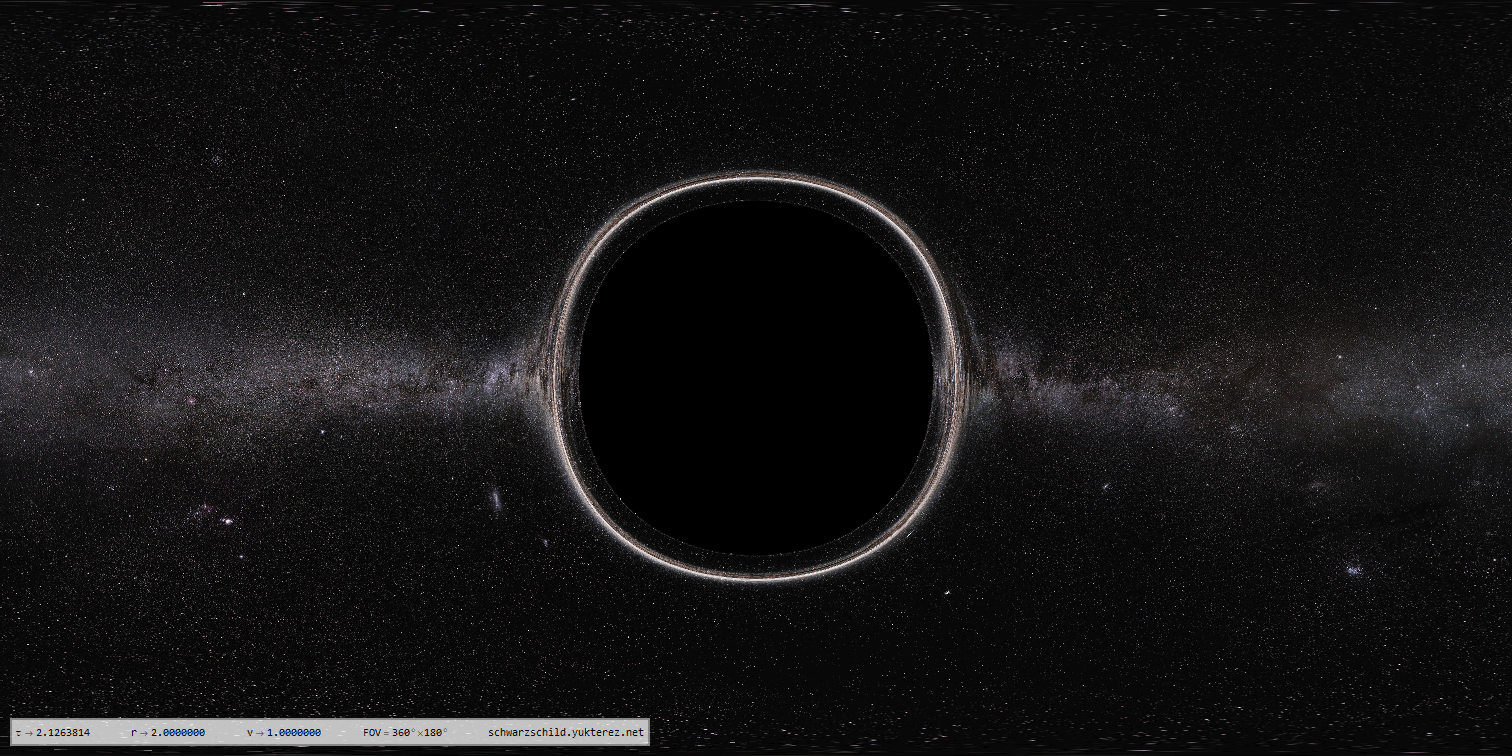
Full panorama of the oberserver falling with the negative escape velocity v=-c√(rₛ/r) when he crosses the event horizon
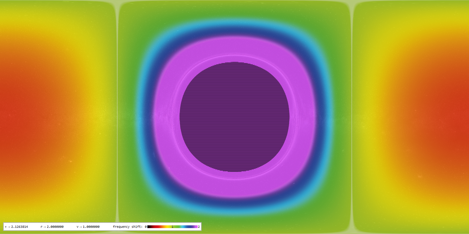
Red/blueshift profile for the observer falling with the negative escape velocity in the image above

Aberration in the eyes of three different observers at the same position r=6GM/c² with different velocity vectors

Optical distortion of a sphere with r=1.0001rₛ, observer at R=17.5rₛ: due to gravitational lensing the back of the sphere is also visible
left: lightrays in flat Minkoswki space, right: Schwarzschild. Distance of the light source to the black hole: 20GM/c²
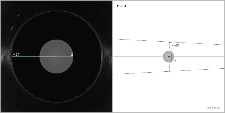
Ray bundle with impact parameter b=√27≈5.2GM/c² (the apparent radius of the black hole from the perspective of the far away observer)
Orbit with perihelion shift; initial conditions: r₀=5, θ₀=π/2, v₀=vz₀=vθ₀=51/50·√((1/5)/(1-2/5)).
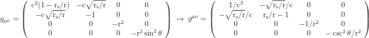
▥ Metric tensor in Schwarzschild coordinates {t,r,θ,φ}:


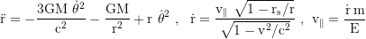
▦ Ingoing Finkelstein coordinates with the horizon penetrating coordinate time dt→dť+dr(rs/r)/(1-rs/r)/c:

▧ Raindrop aka Gullstrand Painlevé coordinates, coordinate time defined by freefallers from infinity, dt→dτ+dr√(rs/r)/(1-rs/r)/c:

Equations of motion in Schwarzschild coordinates (for photons set the gammafaktor to 1, μ=0 and m=hf/c²=constant, where f is the frequency when arriving at infinity):
For a purely radial motion the equation of motion simplifies to
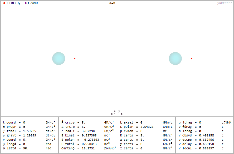
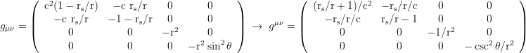
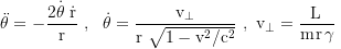
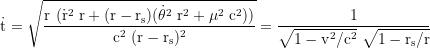
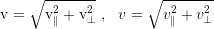
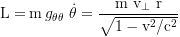
τ is the proper time of the test particle, and t the coordinate time of an observer at infinty. To get the shell time T of a stationary fiducional observer at r=R, t gets multiplied with √(1-rs/r), where rs=2GM/c² is the Schwarzschildradius. The total time dilation is the product of the gravitational and the kinetic component. v⊥=v cos ζ (the transverse), and v∥=v sin ζ (the radial component of the local velocity). ζ is the vertical launch angle (because of the radial length contraction ζ at small r looks flatter when viewed from infinity).
Transformation between local and observed (shapirodelayed) velocities:

With Pythagoras we get the total velocity:
The orbital angular momentum
and the total energy of the test particle in the frame of an observer at infinity
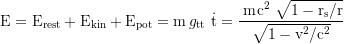
are conserved. The rest, kinetic and potential energy (defined as the difference between local and total energy) are

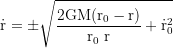
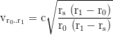
The required radial velocity to get from r₀ to r₁ is
and the escape velocity from r₀ to infinity

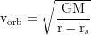
Circular orbit velocity, at the photon sphere at r=3rₛ/2 it is the speed of light:
Free fall time from rest at r₀ to r (proper time):
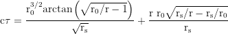
coordinate time for the free fall from r₀ to r:

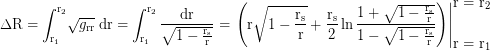
The physical distance between r₁ and r₂ measured with local and stationary rulers is
Distance from the horizon to the singularity in the frame of a freefaller falling in with the negative escape velocity:
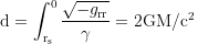
in Droste coordinates with grr=-1/(1-rₛ/r) and v=-√(rₛ/r) where γ=1/√(1-v²/c²) or in Raindrop coordinates with grr=-1 and v=0 where γ=1. In the frame of a freefaller starting from rest at an infinitesimal above the horizon the integrated distance approaches d=πGM/c².
For the simulatior codes and more images and animations see the german version and the article about the relativistic raytracer. Other coordinates: see here
▦ Ingoing Finkelstein coordinates with the horizon penetrating coordinate time dt→dť+dr(rs/r)/(1-rs/r)/c:
▧ Raindrop aka Gullstrand Painlevé coordinates, coordinate time defined by freefallers from infinity, dt→dτ+dr√(rs/r)/(1-rs/r)/c:
Equations of motion in Schwarzschild coordinates (for photons set the gammafaktor to 1, μ=0 and m=hf/c²=constant, where f is the frequency when arriving at infinity):
For a purely radial motion the equation of motion simplifies to
τ is the proper time of the test particle, and t the coordinate time of an observer at infinty. To get the shell time T of a stationary fiducional observer at r=R, t gets multiplied with √(1-rs/r), where rs=2GM/c² is the Schwarzschildradius. The total time dilation is the product of the gravitational and the kinetic component. v⊥=v cos ζ (the transverse), and v∥=v sin ζ (the radial component of the local velocity). ζ is the vertical launch angle (because of the radial length contraction ζ at small r looks flatter when viewed from infinity).
Transformation between local and observed (shapirodelayed) velocities:
With Pythagoras we get the total velocity:
The orbital angular momentum
and the total energy of the test particle in the frame of an observer at infinity
are conserved. The rest, kinetic and potential energy (defined as the difference between local and total energy) are
The required radial velocity to get from r₀ to r₁ is
and the escape velocity from r₀ to infinity
Circular orbit velocity, at the photon sphere at r=3rₛ/2 it is the speed of light:
Free fall time from rest at r₀ to r (proper time):
coordinate time for the free fall from r₀ to r:
The physical distance between r₁ and r₂ measured with local and stationary rulers is
Distance from the horizon to the singularity in the frame of a freefaller falling in with the negative escape velocity:
in Droste coordinates with grr=-1/(1-rₛ/r) and v=-√(rₛ/r) where γ=1/√(1-v²/c²) or in Raindrop coordinates with grr=-1 and v=0 where γ=1. In the frame of a freefaller starting from rest at an infinitesimal above the horizon the integrated distance approaches d=πGM/c².
For the simulatior codes and more images and animations see the german version and the article about the relativistic raytracer. Other coordinates: see here

